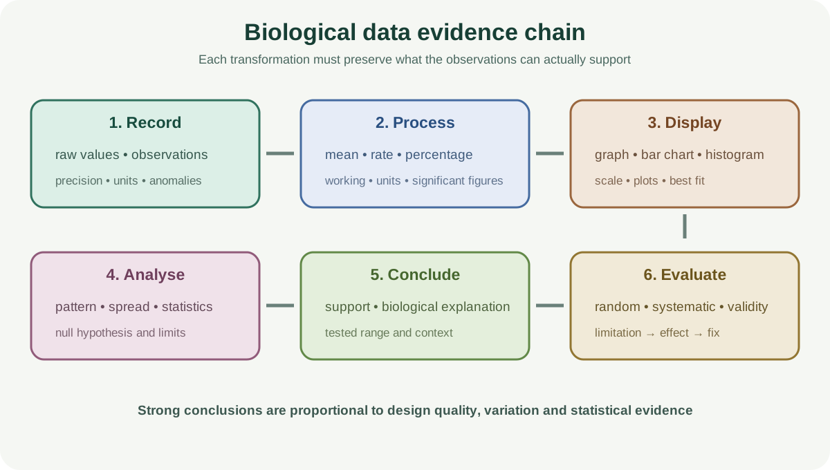
Biological Data Analysis and Evaluation develops the presentation, analysis, conclusion and evaluation skills assessed across Cambridge Biology 9700 Papers 3 and 5. It covers raw records, tables, graphs, calculations, variation, statistical decisions, bounded conclusions, anomalies, error types and targeted improvements. Theory supplies biological explanations; this practical note owns the evidence chain from observations to justified claims.
1. Preserve raw data
Raw data are direct measurements or observations before processing. Record them immediately rather than reconstructing them from memory. Do not replace replicate measurements with a mean or discard an inconvenient value.
Quantitative data need the precision supported by the instrument. Repeated measurements from the same instrument should normally use consistent decimal places. Qualitative observations need specific descriptions, such as colour and distribution, rather than “normal” or “changed.”
Record procedural observations that may explain results, including bubbles, spills, damaged tissue, delayed timing or an instrument reaching its limit.
2. Construct a valid table
Put the independent variable in the left column, or above the dependent variable if the table uses rows. Use descriptive headings with units in the headings and no units in the body cells.
Separate raw replicates from processed means, rates or percentage changes. Keep enough precision in intermediate values to avoid rounding error, then report final calculations appropriately.
Tables should be self-contained. A heading such as “time / s” is clearer than “results.” If two quantities share a unit, each still needs a distinct descriptive heading.
3. Choose the correct display
Use a graph for continuous quantitative data, a bar chart for discontinuous or categorical data and a histogram for frequency data grouped into continuous intervals.
Place the independent variable on x and dependent variable on y. Label axes to match table headings, including units. Select simple scales that use most of the grid and can be read to within half a small square.
Plot small crosses or circled dots accurately. Use a best-fit line, smooth curve or ruled point-to-point connection according to the pattern and instruction. Do not extrapolate unless the evidence and context justify it.
Bar charts have separate bars for distinct categories. Histogram bars touch because class intervals form a continuous scale. Width and frequency density may matter when interval widths differ.
4. Show calculations and precision
Display each calculation with the relationship, substitution, steps and final unit. This allows reasoning marks and makes transcription errors visible.
Check this topic from memory
Attempt the matching topic bank before reopening the notes. Use each missed idea to decide what to review next.
Use the same number of significant figures as, or one more than, the smallest number of significant figures in the source data, following the assessment guidance. Avoid carrying a long calculator display into the reported answer.
Common processing includes means, percentage gain or loss, rates of change, magnification, calibration, gradients and estimates from graphs. Preserve signs where they carry biological meaning.
5. Describe patterns before explaining them
A description identifies direction, shape, threshold, optimum, plateau and anomaly using data. Quote values or ranges to support the statement. “It increases” is incomplete if the pattern later levels or decreases.
An explanation links that pattern to biological mechanisms. Keep the tasks separate: observation first, mechanism second. If the context is unfamiliar and explanatory information is supplied, use it rather than inventing unsupported theory.
Compare datasets directly, including similarities and differences in trend, magnitude, optimum and variation.
6. Use graphs to estimate values
Interpolation estimates within the measured range. Extrapolation predicts outside it and carries greater uncertainty. Show construction lines or explain how a value was read when requested.
For a gradient, choose two well-separated points on the best-fit line or tangent, not necessarily two data points. Calculate vertical change divided by horizontal change and derive the unit from the axes.
An instantaneous rate uses a tangent at the relevant point. A mean rate uses total change divided by total time. Do not switch between them without stating which quantity is required.
7. Summarise variation
A mean estimates the centre of repeated quantitative results. The range describes total spread but is strongly affected by extremes. Standard deviation describes spread of observations around a mean.
Standard error describes uncertainty in the estimated mean and usually decreases as independent sample size grows. A 95 percent confidence interval gives a range constructed to capture the population mean in the stated long-run sense.
Error bars must be identified before interpretation. Standard deviation bars describe sample variation; standard error or confidence intervals address precision of mean estimates. Overlap rules are not universal substitutes for a statistical test.
8. Select a statistical test
Identify the question and data type. A t-test compares two means under the relevant assumptions. Chi-squared compares observed categorical frequencies with expected frequencies. Spearman's rank correlation tests monotonic association using ranks. Pearson's coefficient tests linear association between quantitative variables.
State a null hypothesis of no difference, no association or no departure from expected frequencies as appropriate. Calculate using the supplied formula or method, identify degrees of freedom where required and compare with the critical value or probability threshold.
Rejecting the null hypothesis means the evidence is unlikely under that null at the chosen threshold. It does not prove the biological mechanism or guarantee practical importance. Failing to reject does not prove the groups are identical.
9. Draw a bounded conclusion
Summarise the main pattern and state whether the hypothesis is supported. Use “supports” rather than “proves” because alternative explanations and sampling uncertainty remain.
Tie the conclusion to the tested range, species, tissue, conditions and measurement. A relationship observed between 10 and 50 degrees Celsius cannot be assumed at 80 degrees Celsius.
Use processed data, graph features and statistical evidence together. Then give a biological explanation proportionate to the evidence. If results are inconsistent, state that confidence is limited rather than forcing one decisive claim.
10. Identify anomalous values
An anomaly does not fit the overall pattern or differs substantially from replicates. Identify it using values, then inspect records for a plausible procedural explanation.
Do not delete it automatically. Check calculation and transcription, repeat the treatment if possible and report analyses with transparent handling. If no objective reason exists, retaining it may be more defensible.
An anomaly can reveal genuine biological variation. Calling every unexpected point “human error” neither explains it nor justifies removal.
11. Distinguish random and systematic error
Random error causes unpredictable variation between measurements and can obscure a trend. It can arise from endpoint judgement, biological differences or fluctuating conditions. Independent replicates and improved control help estimate or reduce it.
Systematic error shifts measurements consistently in one direction, such as a miscalibrated balance or incorrect blank. It may leave the trend shape intact while making absolute values inaccurate. More repeats do not remove systematic bias.
An instrument's finite resolution creates measurement uncertainty, not automatically a mistake. State how it affects the particular result.
12. Evaluate validity and confidence
Validity asks whether the investigation tested the hypothesis. Check confounding variables, controls, measurement suitability and whether the independent variable caused unintended changes.
Confidence depends on sample size, replication, spread, anomalies, range, interval, accuracy and repeatability. A narrow range may support a local trend but not an optimum. Wide variation may make a mean difference uncertain.
Separate evidence quality from agreement with prediction. Results that match theory can still come from a weak method; unexpected results can be valid.
13. Suggest targeted improvements
Write a three-part chain: limitation, likely effect and improvement. “Temperature varied, changing enzyme rate unpredictably; use a thermostatically controlled water bath and equilibrate solutions” is stronger than “control temperature.”
Improvements include a more accurate dependent-variable method, more effective standardisation, smaller independent-variable intervals, independent replicates for a mean and spread, calibration, random allocation and appropriate controls.
More data are useful only if they address the weakness. Repeating a systematically biased method produces more precise bias. Name feasible apparatus and procedure rather than “use a machine.”
14. Propose an extension
An extension answers a new question by testing a different independent variable, organism, tissue or condition. State the new variable, range and dependent measurement while retaining relevant controls.
Do not present an extension as a repair. Testing pH after a temperature investigation broadens knowledge but does not fix inconsistent temperature in the original method.
A prediction based on the original conclusion can motivate the extension, but the new investigation still needs its own valid design.
Worked application: analyse an enzyme dataset
Mean enzyme rates at 20, 30, 40, 50 and 60 degrees Celsius are 1.2, 2.1, 3.4, 2.6 and 0.7 arbitrary units per minute. Describe an increase to the highest measured mean at 40 degrees Celsius, followed by a decline. Conclude that the data support an optimum within the tested region, but not that exactly 40 degrees Celsius is the true optimum. Inspect replicate spread and any anomalies, then test smaller intervals from 35 to 45 degrees Celsius. If one 40-degree replicate is unusually high, check records and repeat independently rather than deleting it. Use controlled pH, substrate and enzyme preparation to strengthen causal interpretation.
Common misconceptions and corrections
Recording only means. Preserve raw replicates.
Putting units in every data cell. Put units in headings.
Using inconsistent decimal places for one instrument. Match its precision.
Calling arbitrary categories continuous data. They may be ordinal or nominal.
Using a bar chart for a continuous variable. Use a graph.
Separating histogram bars. Continuous class intervals touch.
Using a tiny graph scale. Use most of the grid with readable intervals.
Drawing a line beyond all data automatically. Avoid unsupported extrapolation.
Reporting calculator precision. Match significant figures to source data.
Describing a pattern without values. Quote evidence.
Explaining before describing. Establish the observed pattern first.
Using data points instead of a tangent. Instantaneous rate needs the tangent.
Calling standard deviation uncertainty in the mean. Standard error serves that role.
Treating all error-bar overlap identically. Identify the error measure and test.
Choosing statistics by familiarity. Match question and data type.
Saying significance proves causation. Design and controls remain essential.
Saying non-significance proves equality. Evidence may be insufficient.
Writing that results prove a hypothesis. They support it within limits.
Generalising beyond the tested range. Bound the conclusion.
Deleting every anomaly. Investigate and report transparently.
Writing “human error.” Name the mechanism and effect.
Calling random scatter systematic. The two error types differ.
Adding repeats to fix calibration bias. Recalibrate the instrument.
Equating agreement with theory to validity. Method quality is independent.
Suggesting “more accurate equipment” vaguely. Name it and the error reduced.
Calling a new variable an improvement. It is an extension.
Assessment guidance
Build every answer around the evidence chain. Preserve raw data, use correctly headed tables and select a display from data type. Show calculations, units and sensible precision. Describe patterns with quoted values before explaining them. Statistical answers require a matched test, null hypothesis and bounded decision. Conclusions should state support and limitations, not proof. Identify anomalies explicitly and distinguish random variation from systematic bias. Evaluation earns marks when each limitation has a likely effect and feasible improvement. An extension needs a new question and variables; it does not repair the original investigation.
Retrieval practice
Correct three flawed data tables and choose displays for continuous, categorical and frequency data. Calculate a mean, percentage change, rate and tangent gradient with units and precision. Describe and explain two unfamiliar graphs. Match four datasets to t-test, chi-squared, Spearman and Pearson and write null hypotheses. Classify errors as random or systematic, handle three anomalies transparently and turn six vague evaluation statements into limitation-effect-improvement chains. Finish with one bounded conclusion and one genuine extension.