Cambridge International AS and A Level Chemistry Practical 2: Rates and Kinetics Investigations
Cambridge International AS and A Level Chemistry Practical 2: Rates and Kinetics Investigations
Study guide/
Cambridge International Chemistry 9701 practical notes on clock and continuous-rate methods, initial gradients, variables, temperature control, graphs, uncertainty and evaluation.
Rates and Kinetics Investigations is the second Cambridge Chemistry 9701 practical-skills note. It applies Paper 3 timing, measurement, graphing and evaluation expectations and Paper 5 planning skills to clock reactions, gas or mass monitoring, initial rates, concentration changes and temperature control. The rate-equation theory remains in the theory hub.
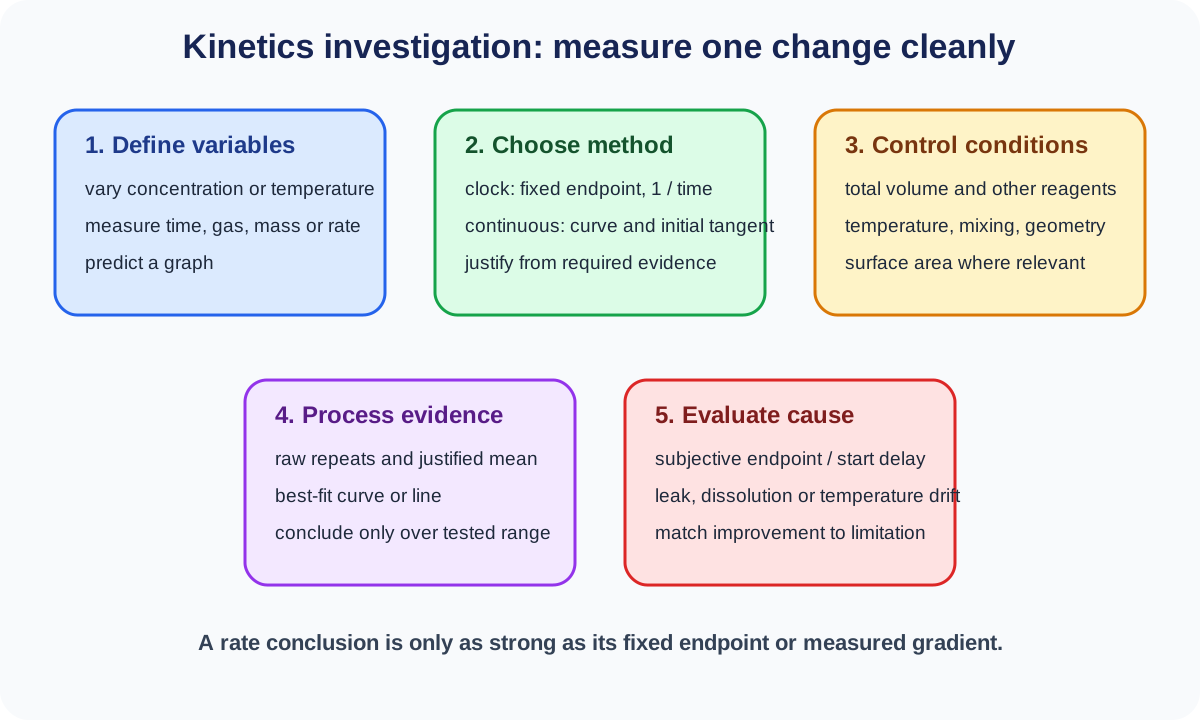
1. Define the experimental question
State how one independent variable affects a measurable dependent variable. Typical independent variables are concentration or temperature; the dependent variable may be time to a fixed endpoint, gas volume, mass or calculated rate.
Name the chemical system and range. “Investigate rate” is too vague to determine apparatus or analysis.
The prediction may be expressed in words or as a sketched graph, but it must match the chosen measurement.
2. Clock method principle
A clock method measures time until the reacting system reaches a fixed visible condition. Cambridge names acidified sodium thiosulfate obscuring printed material through sulfur formation as an example.
If every run uses the same endpoint amount, rate is proportional to reciprocal time. Shorter time indicates faster rate.
The method gives an average proxy to a fixed extent, not a complete concentration-time curve.
3. Disappearing-cross method
Place the reaction vessel over the same printed cross, mix reagents and start timing immediately. Stop when the cross is first no longer visible through the suspension.
Use the same flask, liquid depth, cross, lighting, viewing position and observer. These control how much precipitate is needed to obscure the mark.
The endpoint is subjective, so repeats and a consistent observer reduce random scatter.
4. Other clock endpoints
A colour appearance, colour disappearance or sudden iodine-starch signal may provide a fixed endpoint. The chemistry must ensure each run reaches the same reaction extent when the signal changes.
Keep indicator or clock-reagent amounts constant unless they are the independent variable. Explain why the endpoint corresponds to a fixed amount.
Do not use reciprocal time if the endpoint quantity changes between runs.
5. Continuous gas-volume monitoring
Collect gas in a gas syringe and record volume at regular time intervals. Check the apparatus is gas-tight, the syringe moves freely and its capacity exceeds the expected volume.
Start timing at mixing and fit the bung promptly. Gas produced before sealing is lost and makes early volume readings too low.
Check this topic from memory
Attempt the matching topic bank before reopening the notes. Use each missed idea to decide what to review next.
The initial gradient of gas volume against time measures initial gas-formation rate.
6. Continuous mass-loss monitoring
Place a reaction that releases gas on a balance and record mass at regular intervals. A loose cotton plug may prevent spray while allowing gas to escape.
This avoids gas-syringe friction or leaks but is unsuitable if volatile liquids or spray also leave, because their mass loss would be misattributed to product gas.
Use the same balance and record at its supported precision.
7. Choosing between methods
Use a clock method for rapid comparative screening with a clear repeatable endpoint. Use continuous monitoring when curve shape, initial gradient or total product amount matters.
Gas volume is chemically direct but vulnerable to leakage; mass loss is simple but responds to every escaping material. Select by product properties, timescale and precision.
Justify the choice through the evidence required, not apparatus familiarity.
8. Varying concentration by dilution
Prepare a series whose reactant concentration changes while total reaction volume remains constant. Replace removed reactant solution with deionised water.
Final reaction concentration equals stock concentration multiplied by its volume divided by total mixed volume. Use this final value on graphs.
Keeping total volume constant preserves liquid depth and concentrations of other components when their delivered amounts remain fixed.
9. Range and spacing
Choose at least five suitably spaced independent-variable values where feasible. The range should be wide enough to expose the relationship but safe and measurable.
Very fast runs have large timing percentage uncertainty; very slow runs waste time and may introduce drift. A preliminary trial can refine the range.
Closer spacing may be useful near a suspected change or graph feature.
10. Temperature control
Use a thermostatically controlled water bath where possible. Bring each reactant solution to the target temperature before mixing and verify temperature rather than assuming bath setting equals solution temperature.
Keep volumes, concentrations, apparatus and mixing constant. Begin reaction only after thermal equilibration.
For an exothermic or long reaction, monitor whether temperature changes during the run and evaluate that limitation.
11. Mixing and timing zero
Define a reproducible mixing sequence. Add the final reagent rapidly, start the timer at the same event and mix in the same manner for every run.
Manual start delay matters most for fast reactions. Video analysis, data logging or slower conditions may reduce the relative delay.
Do not claim a human is the error; identify reaction-time delay or subjective endpoint as the measurable limitation.
12. Controlled variables
Control all variables that can change rate or measured endpoint: other reactant concentrations, total volume, temperature, catalyst amount, particle surface area, mixing, apparatus geometry and observation conditions.
Explain how each important control is maintained and why it matters. Listing temperature as controlled without a water bath or monitoring method is incomplete.
A control experiment may test whether the independent variable, rather than another factor, causes the response.
13. Solid reactants
When using a solid, control mass, purity and surface area. Equal masses of powder and chips do not offer equal exposed area.
Sieve particles into a defined size range or use material from the same prepared batch. Add the solid through a reproducible method that does not delay sealing.
Surface-area variation can create random scatter or a systematic comparison bias.
14. Raw-data table
Prepare the table before collecting data. Put units in headings and record independent-variable values, time and all continuous readings at consistent precision.
Keep repeats as separate raw values, then include a processed mean or rate column. Do not replace raw measurements with averages.
Record qualitative observations such as delayed cloudiness or unusual bubbling because they may explain anomalies.
15. Repeats and anomalies
Repeat each condition sufficiently to estimate variability. Calculate a mean from consistent trials and identify anomalous readings rather than deleting them silently.
Repeat an anomalous condition to test whether the deviation persists. Report the rule used to exclude any value.
Repeats reduce random uncertainty but do not repair a leaking apparatus or wrong concentration series.
16. Reciprocal-time processing
For a valid fixed-endpoint clock, calculate one divided by time as a relative rate. Its unit is inverse seconds when time is in seconds.
The proportionality constant depends on the fixed amount required to trigger the endpoint, so reciprocal-time values are best for comparisons within the same method.
Do not label reciprocal time as an absolute concentration-per-time rate unless the endpoint amount is quantified.
17. Continuous curve and initial gradient
Plot product amount or reactant amount against time. Draw a smooth best-fit curve and identify anomalies.
Find initial rate from a tangent at time zero. Choose two well-separated points on the tangent, not two adjacent raw points, and include graph-scale units.
Later gradients decrease as reactants are consumed or products accumulate.
18. Comparing concentration effects
Plot relative or initial rate against final reactant concentration while other conditions remain controlled. The shape provides experimental evidence for concentration dependence.
For a proposed linearisation, calculate the transformed variable explicitly and use appropriate axes. Do not force a straight line by ignoring curved data.
State the tested range and avoid extrapolating beyond it without justification.
19. Comparing temperature effects
Plot measured rate or reciprocal time against temperature only when the investigation asks for an empirical trend. A graph against reciprocal absolute temperature or logarithmic rate needs theoretical justification and supplied expectations.
Convert Celsius to kelvin when a reciprocal-temperature analysis requires absolute temperature.
Conclude from the observed range rather than claiming a universal doubling rule.
20. Timing uncertainty
Stopwatch resolution may be small, but human start and endpoint response can dominate. Estimate an uncertainty consistent with the actual procedure.
Percentage timing uncertainty is larger for short times. Slowing the reaction or using automated detection can reduce the fractional effect.
Repeats expose response scatter but do not eliminate a consistent start delay.
21. Gas-method limitations
Leaks and delay in fitting the bung make recorded gas volumes too low, especially early in the reaction. Gas dissolving in the mixture can also lower collected volume.
A sticking syringe adds resistance and can distort readings. Test gas-tightness beforehand and use suitable low-friction equipment.
Trace whether each problem affects gradient, final volume or both.
22. Clock-method limitations
The disappearing-cross endpoint depends on eyesight, lighting and viewing angle. Increasing cloudiness may not correspond perfectly to the same amount when liquid depth or particle formation changes.
Use a light sensor or colorimeter for an objective threshold where appropriate. Keep geometry and threshold fixed.
This improvement targets endpoint subjectivity; it does not correct incorrect concentrations.
23. Safety and disposal
Assess each reagent and product. Acidified thiosulfate can release sulfur dioxide, so use small quantities and good ventilation or a fume hood where risk assessment requires it.
Avoid sealed systems when uncontrolled gas pressure can build, except apparatus designed to measure gas safely. Wear eye protection and secure glassware.
Link each hazard to exposure route and a specific control.
Worked application: concentration and clock-rate evidence
Five mixtures use 10.0, 8.0, 6.0, 4.0 and 2.0 cubic centimetres of 0.200 moles per cubic decimetre thiosulfate, with water added so thiosulfate plus water always totals 10.0 cubic centimetres. Each receives the same acid volume at the same temperature. Mean obscuring times are 20.0, 25.1, 33.5, 50.2 and 100.4 seconds. Reciprocal times are proportional to 0.0500, 0.0398, 0.0299, 0.0199 and 0.00996 inverse seconds, closely tracking the final thiosulfate concentration. This supports direct proportionality over the tested range. It does not prove a complete mechanism, and the subjective visual endpoint should be evaluated with repeats or replaced by a fixed light-sensor threshold.
Common misconceptions and corrections
Calling time itself the rate. For a fixed endpoint, relative rate is proportional to reciprocal time.
Using reciprocal time when endpoint quantity changes. Keep the threshold constant.
Claiming a clock method gives a full rate curve. It gives one time to fixed extent.
Changing flask shape between cross trials. Liquid depth changes the endpoint.
Changing observers without control. Visual thresholds can differ.
Using gas collection without leak testing. Product may escape.
Fitting the bung slowly. Early gas loss biases initial rate.
Using mass loss with a volatile reagent. Non-product evaporation confounds data.
Choosing a method without linking it to evidence. Curve and endpoint questions need different data.
Diluting reactant without keeping total volume fixed. Other concentrations and depth can change.
Plotting stock concentration instead of mixed concentration. Use final reaction concentration.
Choosing only two concentrations. A relationship needs a useful range.
Using extremely fast trials. Start-delay percentage uncertainty becomes large.
Assuming bath temperature equals solution temperature. Equilibrate and measure.
Changing mixing intensity between runs. It alters early reaction conditions.
Writing human error. Name timing delay or endpoint judgement.
Calling a variable controlled without a method. State how it is held constant.
Keeping solid mass but changing particle size. Surface area changes.
Averaging before recording raw repeats. Preserve every measurement.
Deleting anomalies silently. Investigate and justify treatment.
Saying repeats fix a leak. They address random variation, not systematic loss.
Giving reciprocal time concentration-rate units. Its direct unit is inverse time.
Taking initial gradient from two early raw points. Draw a time-zero tangent.
Using a tiny gradient triangle. Use widely separated tangent points.
Forcing a straight line through curved data. Follow the evidence.
Claiming rate always doubles per ten degrees. Test the actual range.
Using Celsius in reciprocal-temperature work. Use kelvin.
Treating stopwatch resolution as the only uncertainty. Response time may dominate.
Proposing a colorimeter without a threshold. Define the same objective endpoint.
Sealing a gas-producing reaction in unsuitable glassware. Control pressure safely.
Assessment guidance
Paper 3 answers should show reproducible mixing, immediate timing, precise raw tables, a suitable number and range of readings, repeat handling and correct graph technique. Use reciprocal time only for a fixed endpoint, and use a time-zero tangent for continuous initial rate. Paper 5 plans must define independent, dependent and controlled variables, final concentrations, apparatus, timing event, temperature equilibration, safety and intended processing before data collection. Evaluation should distinguish subjective endpoints, start delay, leakage, dissolution, temperature drift and surface-area variation, then match each cause to its likely direction, random or systematic character and a realistic improvement.
Retrieval practice
Plan the same concentration investigation once with a disappearing cross and once with continuous gas collection, then compare what each method can conclude. Calculate final mixed concentrations and reciprocal times, draw an initial tangent and derive its units. Design a temperature series with pre-equilibration and controls. Finish by diagnosing datasets containing an anomalous repeat, a gas leak, a changing solid surface area and trials too fast for manual timing.
Cambridge International, Chemistry 9701 syllabus for examinations in 2025, 2026 and 2027, Practical Assessment section for Paper 3 rates experiments, measurement, graphing, analysis and evaluation, and Paper 5 planning, dealing with data, conclusions and evaluation.