Cambridge International AS and A Level Marine Science Practical Skills 6: Descriptive statistics and statistical tests
Cambridge International AS and A Level Marine Science Practical Skills 6: Descriptive statistics and statistical tests
Study guide/
Cambridge Marine Science 9693 practical notes on averages, spread, Lincoln and Simpson indices, Spearman correlation, error bars and chi-squared tests.
Descriptive Statistics and Statistical Tests develops the official Cambridge International AS and A Level Marine Science 9693 quantitative analysis boundary. Mean, median, mode, range, Spearman's rank, the Lincoln index and Simpson's index can be assessed at AS and A Level. Standard deviation, standard error, 95 per cent confidence intervals and chi-squared are A Level additions. Statistics summarise evidence or test a defined hypothesis; they do not rescue a biased design.
Official assessment boundary
Paper 2 can assess mean, median, mode, range, Spearman's rank correlation, the Lincoln population estimate and Simpson's index of diversity. Paper 4 can assess all of these plus standard deviation, standard error, 95 per cent confidence intervals and chi-squared.
Formulae and statistical-test symbols are supplied when needed, except the number of chi-squared degrees of freedom, which candidates must know. Questions may provide partly completed calculations.
The syllabus does not expect candidates to distinguish population from sample standard-deviation formula conventions. Focus on correct substitution, interpretation and method assumptions.
Begin with question and data type
Ask what the investigation needs:
a typical value
spread or precision
a population estimate
diversity comparison
evidence of monotonic correlation
evidence that observed nominal frequencies differ from expectation
Then check that sampling units are independent and representative. A correct calculation on pseudoreplicated or biased data produces a precise-looking but weak conclusion.
State a null hypothesis before a significance test and return to it after using the critical value or probability information.
Mean
The arithmetic mean is total of the values divided by number of values. It uses every observation and works well as a centre for roughly balanced numerical data.
An extreme value can shift the mean strongly. Inspect raw data and justify treatment of anomalies before calculation.
Keep unrounded values until the final result and include the measured quantity's unit.
A mean without sample size or spread does not show reliability.
Median
The median is the middle value after ordering the data. For an even number of values, it is the mean of the two central values.
It is less affected by extremes and can be useful for skewed abundance or size data. It does not use the magnitude of every observation in the same way as the mean.
Check this topic from memory
Attempt the matching topic bank before reopening the notes. Use each missed idea to decide what to review next.
The median's unit is the same as the original measurement.
Mode
The mode is the most frequent value or category. It can describe numerical or categorical data.
A dataset can have more than one mode or no unique mode. Grouped modes depend on class boundaries.
Mode is useful for common shell-size class or dominant category but may ignore most of the distribution.
Do not calculate it by adding or dividing values.
Range
Range is maximum minus minimum. It gives a simple measure of spread at AS and A Level.
It depends only on two observations and tends to grow as sample size increases, so compare it cautiously across unequal samples.
An anomaly can inflate range greatly. Retain the raw value and justify any exclusion.
Range has the same unit as the data.
Choosing a centre and spread
Use mean with a spread measure when data and question justify it. Use median when skew or valid extremes make the mean unrepresentative. Use mode for most common value or category.
Explain the choice from the distribution, not from which answer looks more favourable.
At AS Level, mean or median with range may describe centre and variation. At A Level, standard deviation can give a fuller measure of spread around the mean.
No summary replaces the raw pattern or graph.
Lincoln index for mark-release-recapture
The Lincoln estimate is:
N=m2n1n2
Here, N is estimated population size, n1 is the first marked sample, n2 is the total second sample and m2 is marked individuals recaptured.
The estimate assumes marks remain and are recognised, marking does not alter survival or catchability, marked organisms mix fully, sampling periods are short enough for a closed population, and every individual has similar capture probability.
A very small recapture count makes the estimate unstable. Zero recaptures makes the formula unusable.
Interpreting Lincoln bias
If marked organisms become trap-shy, too few are recaptured, so the denominator is too small and population size is overestimated. If marked organisms are attracted to traps, recaptures rise and the estimate may be too low.
Immigration of unmarked organisms can reduce marked proportion and inflate the estimate. Mark loss has a similar effect.
Mortality or emigration of marked individuals changes the population and recapture pool.
State the direction through the formula rather than labelling an assumption merely "unreliable".
Simpson's index of diversity
The syllabus form is:
D=1−∑(Nn)2
Here, n is the number of individuals of each species and N is the total number of individuals across species.
The index combines richness and evenness. In this form, a larger value indicates greater diversity because dominance by one species makes the squared-proportion sum larger and D smaller.
Compare sites only when sampling effort, identification and detectability are sufficiently comparable.
Richness, evenness and sampling
Species richness is number of species. Evenness is how similarly individuals are distributed among species.
Two sites can have equal richness but different Simpson values if one is dominated by a single species. Rare species contribute little to abundance-weighted indices but may still matter ecologically.
Larger sampling effort often detects more species. Standardise area, time, mesh, tide and identification method.
An index is a summary of the sampled community, not proof that every habitat function is healthy.
Spearman's rank correlation
Spearman's rank tests monotonic association between paired variables that are ordinal or can be ranked. The supplied formula is:
rs=1−n3−n6∑D2
Here, D is the difference between paired ranks and n is number of pairs.
The official guidance expects independent points, random selection, a scatter pattern suggesting an increasing or decreasing relationship and usually 10 to 30 pairs, although the test can be used with more than five.
Ranking and tied values
Rank each variable consistently in the same direction. For tied values, assign the mean of the ranks they would occupy.
Keep original pairs together after ranking. Calculate rank difference and its square for every pair.
A small squared-rank-difference sum gives rs near positive one; opposing ranks give a negative value.
Check that rank totals match the expected sum to find ranking errors.
Spearman interpretation
Values range from negative one for perfect negative correlation through zero for no monotonic correlation to positive one for perfect positive correlation.
Magnitude alone does not establish statistical significance. Compare the calculated value with the supplied critical value for sample size and chosen probability level according to the table rule.
If significant, reject the null hypothesis of no correlation. Then describe direction and context.
Correlation does not prove that one variable causes the other; a third variable or reverse relationship may exist.
Standard deviation at A Level
Standard deviation describes spread of observations around the mean. The supplied formula uses deviations, squares and sample size.
A smaller standard deviation means values are more tightly clustered around their mean when units and scale are comparable. It does not show whether the mean is accurate.
One extreme value can increase standard deviation. Sample design and distribution should be inspected.
Standard deviation has the same unit as the original variable.
Standard error at A Level
Standard error describes precision of the sample mean as an estimate. The supplied relationship is:
SE=ns
It decreases as sample size increases when standard deviation is comparable. It is smaller than standard deviation for samples larger than one.
Standard error does not describe the spread of individual organisms and does not correct sampling bias.
Report it with the same unit as the mean.
95 per cent confidence interval at A Level
The syllabus uses the approximation:
95%,CI=xˉ±2(SE)
This gives a range around the sample mean for the population mean under the method's assumptions.
Narrower intervals indicate a more precise mean estimate. They do not mean 95 per cent of individual observations lie inside.
Compare intervals together with independence, sample size and design. Do not use non-overlap as an infallible universal significance test.
Error bars
Plot mean at the point or bar height and extend bars by the stated statistic. A standard-error bar runs one SE above and below unless the prompt says otherwise; a confidence-interval bar reaches the interval limits.
Label or state what bars represent. Do not mix SD and SE among treatments.
Long bars show greater spread or lower mean precision according to the statistic used.
Graph scale must allow bar endpoints to be read accurately.
Chi-squared test at A Level
Chi-squared tests whether observed nominal frequencies differ significantly from expected frequencies. The supplied formula is:
χ2=∑E(O−E)2
For each category, subtract expected from observed, square, divide by expected and sum. The syllabus limits expected examination calculations to one row or one column of data.
The data are counts in mutually exclusive categories, observations are independent and expected frequencies must be suitable for the test guidance supplied.
Expected frequencies and null hypothesis
Expected values come from the stated theoretical ratio, equal distribution or relevant model, not from copying the observations.
A null hypothesis might be: there is no significant difference between observed habitat counts and the expected distribution.
Expected frequencies should sum to the same total as observed frequencies. If they do not, the setup is wrong.
Chi-squared uses counts, not percentages or means substituted into the formula without converting to valid expected counts.
Degrees of freedom and critical values
For the one-dimensional class comparison required here:
v=c−1
where c is number of classes. This formula must be recalled.
Use degrees of freedom and the stated probability level to find the supplied critical value. If calculated chi-squared exceeds the critical value under the table convention, reject the null hypothesis; otherwise do not reject it.
"Do not reject" is not proof that observed and expected distributions are identical.
Chance, significance and effect size
A significance test estimates whether the pattern is unlikely under the null model. It does not measure ecological importance directly.
Large samples can make a small difference statistically detectable. Small samples may lack power to detect an important effect.
Report the actual pattern, statistic, decision and biological context. Avoid claiming certainty from one threshold.
Statistical validity still depends on sampling independence, suitable categories and honest data handling.
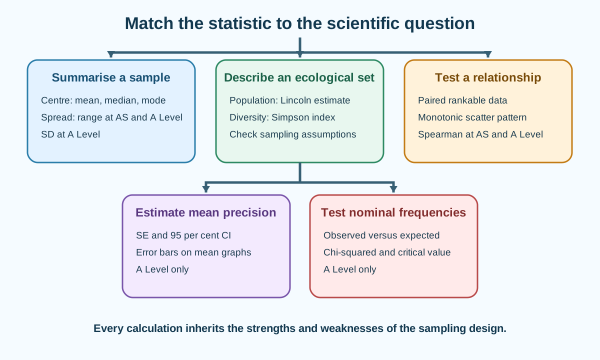
Choosing among the official methods
Use:
mean, median, mode and range to summarise centre or spread
Lincoln index to estimate a marked population
Simpson's index to compare sampled diversity
Spearman's rank to test monotonic association in paired rankable data
SD to describe observation spread at A Level
SE or 95 per cent CI to describe mean precision at A Level
chi-squared to test observed versus expected nominal frequencies at A Level
Do not choose a test merely because its formula is provided.
Worked application: selecting and interpreting statistics
A Paper 4 study records limpet counts and shore height at twelve random independent positions, then classifies 80 snails between two habitat categories with an expected 1:1 distribution. Use mean and standard deviation to summarise limpet abundance, but use Spearman's rank for the monotonic height-abundance relationship after checking the scatter plot and ranking ties. State a null hypothesis of no significant correlation and compare calculated rs with the supplied critical value. For snail habitat, expected counts are 40 and 40. Calculate each (O−E)2/E contribution, sum chi-squared and use one degree of freedom. Compare with the supplied critical value before rejecting or not rejecting the frequency null hypothesis. Neither test proves shore height or habitat alone causes the pattern; sampling, tide and substrate remain relevant.
Common misconceptions and corrections
Calling the mean the most frequent value. That is the mode.
Finding the median without sorting. Order the data first.
Calling range maximum plus minimum. It is maximum minus minimum.
Using mean alone to claim reliability. Spread and sample design matter.
Choosing the statistic that supports the prediction. Choose from data and question.
Using Lincoln index without marked recaptures. Zero makes the estimate unusable.
Assuming marked organisms mix instantly. Mixing is an assumption to evaluate.
Saying trap-shy behaviour underestimates population. Fewer recaptures inflate the estimate.
Ignoring mark loss. It reduces recognised recaptures.
Calling Simpson's index species richness only. It includes evenness.
Assuming identical richness means identical diversity. Dominance can differ.
Comparing diversity under unequal effort automatically. Standardise sampling.
Using Spearman for unpaired data. Each observation needs a pair.
Ranking the two variables in opposite directions accidentally. Use one convention.
Giving tied observations arbitrary consecutive ranks. Use mean rank.
Calling rs=0.8 significant without a critical value. Sample size and threshold matter.
Calling correlation causation. Alternative mechanisms remain.
Calling standard deviation uncertainty in the mean. Standard error serves that role.
Calling standard error spread among organisms. It is mean precision.
Saying larger sample always lowers SD. It does not guarantee less biological spread.
Saying a confidence interval contains 95 per cent of observations. It concerns the mean estimate.
Calling any overlapping intervals no difference. Interpretation is not an absolute visual rule.
Plotting error bars without identifying the statistic. Meaning is ambiguous.
Using chi-squared on continuous measurements directly. It tests nominal counts.
Using percentages in place of expected frequencies. Convert to counts.
Letting expected totals differ from observed totals. The model setup is inconsistent.
Forgetting to square observed-minus-expected. Contributions cannot remain signed.
Dividing by observed instead of expected. The supplied formula uses expected.
Using number of classes as degrees of freedom. For this case it is classes minus one.
Rejecting the null when calculated value is below critical. Follow the supplied table rule.
Accepting the null as proven. Use "do not reject".
Calling statistical significance ecological importance. Effect size and context differ.
Applying a correct test to pseudoreplicates. Design invalidity remains.
Memorising formulae but not assumptions. Test selection and interpretation earn meaning.
Assessment guidance
State the question, data type and null hypothesis before selecting a method. At AS Level, own mean, median, mode, range, Lincoln, Simpson and Spearman; reserve SD, SE, confidence intervals and chi-squared for A Level. Show substitution and intermediate steps with guard digits, then report a justified final precision. For Lincoln and Simpson, explain sampling assumptions and bias direction. For Spearman, preserve pairs, average tied ranks and use the supplied critical value. For chi-squared, use nominal counts, correct expected totals, recall degrees of freedom as classes minus one and compare with the supplied table. Finish with a contextual conclusion that separates statistical significance, causation and ecological importance.
Retrieval practice
Given six marine datasets, select and justify a centre, spread, population estimate, diversity index, correlation test or frequency test. Complete one Lincoln and one Simpson calculation, rank tied Spearman pairs, interpret a critical value, calculate SD, SE and a confidence interval from supplied formulae, then complete a one-row chi-squared test with degrees of freedom. For every result, audit independence, sampling bias and biological meaning.