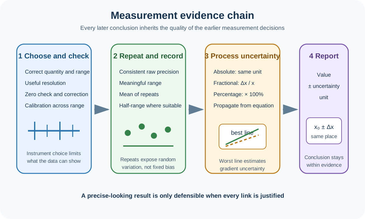
Measurement, calibration and uncertainty form the evidence foundation for Cambridge International AS and A Level Physics 9702 practical work. Paper 3 requires accurate measurements, suitable repeats and justified uncertainty estimates. Paper 5 extends this into absolute uncertainties beside table values, uncertainty propagation, error bars, worst acceptable lines and an uncertainty in the final constant.
Official practical boundary
Paper 3 is a laboratory paper assessing manipulation, measurement and observation; presentation of data and observations; and analysis, conclusions and evaluation. Candidates use common apparatus, analogue scales and digital displays, collect an appropriate range and quantity of data, repeat readings where appropriate, and estimate measurement uncertainty.
Paper 5 is a written planning, analysis and evaluation paper. It assumes practical experience and requires fit-for-purpose measurement choices, possible calibration curves, uncertainty processing and a final result written as value, uncertainty and unit.
The practical questions may use unfamiliar physics. The additional information needed is supplied because the assessment target is experimental skill, not recall of an unlisted theory topic.
Choose a fit-for-purpose instrument
Start with the physical quantity, expected range and change that must be resolved. The instrument must measure the correct quantity, cover the range without overload and have enough resolution to distinguish meaningful changes.
A millimetre rule may suit a long extension but not a thin wire diameter. A micrometer can resolve a small diameter, while calipers can measure an internal or external dimension over a wider range. A top-pan balance measures mass, a newton meter measures force, and an electrical meter must be connected and ranged for the intended current or potential difference.
Resolution is the smallest displayed scale division or digital increment. It constrains what can be read, but it is not automatically the complete uncertainty. Parallax, alignment, a fluctuating display, an indistinct endpoint and sample variation can require a larger justified estimate.
Choose a range that avoids overload while using a substantial part of the scale. A measurement buried in the smallest corner of a broad range usually has poor fractional resolution. For a digital meter, begin safely on a high range if the magnitude is unknown, then reduce the range when safe and useful.
Read analogue and digital instruments
Read an analogue scale with the eye normal to the scale and pointer. This reduces parallax. Identify the value represented by one division before estimating a reading. Record all readings in one raw-data column to the same degree of precision when the instrument and method are unchanged.
Check this topic from memory
Attempt the matching topic bank before reopening the notes. Use each missed idea to decide what to review next.
For a digital display, wait for a stable value or define a repeatable rule for a fluctuating value. Do not invent digits beyond the display. A final digit that changes is evidence of variation and should inform repeats or uncertainty, not be silently discarded.
Place a ruler close to the object and align it with the measured direction. If the object does not begin at zero, subtract the two endpoint readings. This protects the measurement from a damaged zero edge and makes both readings explicit.
Time several consecutive oscillations rather than one when the motion is periodic. Dividing the total time by the number of oscillations reduces the fractional effect of reaction time, provided the same phase point is used at the start and finish.
Check zero and calibration
A zero error is a systematic offset visible when the true input should be zero. Close a micrometer gently and check whether it reads zero. Disconnect or null a sensor only as the stated apparatus permits. Record the sign of any correction: if an instrument reads above zero with no input, subtract that offset from later readings.
Calibration compares instrument response with known reference inputs. A single zero check tests one point; it does not prove correct scale factor across the full range. When a response is not directly in the required physical quantity, collect reference pairs and construct a calibration curve. Interpolate within the calibrated range rather than assuming an unjustified formula.
Calibration cannot remove every uncertainty. Reference values have their own uncertainty, readings may scatter and the device response may drift with temperature or time. Check calibration under conditions close to those of the experiment and state any remaining limitation.
Separate random and systematic effects
Random effects make repeated readings vary unpredictably. Reaction time, changing alignment, electrical noise and judging a blurred boundary can contribute. Repeats reveal this variation. Where appropriate, use the mean as the best estimate and half the range as the absolute uncertainty in a repeated measurement:
Δx=2xmax−xmin.
Systematic effects shift readings in a consistent way. Zero offset, a stretched scale, a miscalibrated sensor or persistent heat loss may cause them. Repeating the same biased method does not remove the shift. Use a zero correction, calibration, comparison method or redesigned procedure matched to the identified cause.
Precision describes how closely repeated values agree. Accuracy describes closeness to the accepted or true value. A tightly clustered set can be precise but inaccurate if a systematic error shifts every result.
Record precision honestly
Build the results table before collecting data. Put the quantity and unit in each heading, for example I/mA, rather than writing a unit beside every entry. Keep raw readings at the precision supported by the same instrument.
For multiplication or division, Cambridge accepts a calculated value with the same number of significant figures as the least precise measured factor, or one more. Do not round intermediate values so early that useful information is lost. Retain guard digits during processing, then round the reported result and uncertainty coherently.
An uncertainty should normally have one significant figure, or sometimes two when needed to avoid excessive rounding. The value should be rounded to the same decimal place as its absolute uncertainty. The required form is
x=(x0±Δx),unit.
Convert and propagate uncertainties
Absolute uncertainty has the same unit as the measured quantity. Fractional uncertainty is Δx/x, and percentage uncertainty is
xΔx×100%.
Convert from percentage to absolute uncertainty by multiplying the percentage fraction by the measured value.
For a sum or difference, add the absolute uncertainties. For a product or quotient, add percentage or fractional uncertainties. If a measured factor is raised to a power, its percentage contribution is multiplied by the magnitude of that power. These rules give a conservative simple estimate within the 9702 boundary.
Write the equation before assigning uncertainty contributions. This prevents mixing an absolute uncertainty in one variable with a percentage uncertainty in another. Keep units attached to absolute uncertainties and omit units from fractions and percentages.
Use uncertainty in graph evidence
Paper 3 requires a sensible range, accurately plotted points and a best-fit trend. A gradient should use two points on the line separated by more than half its length, not two raw data points chosen merely because they are convenient.
Paper 5 can require absolute uncertainties in the table, error bars in both directions where appropriate, and a worst acceptable straight line. The worst acceptable line is the steepest or shallowest line that remains consistent with all error bars. Distinguish it clearly from the best-fit line.
Estimate gradient uncertainty using
Δm=∣mbest−mworst∣.
Use the analogous difference for an intercept. Then carry this uncertainty through the stated relationship to the required constant and report the constant with value, uncertainty and unit.
Worked application: diameter to cross-sectional area
A wire diameter is measured six times in different orientations: 0.48, 0.50, 0.49, 0.51, 0.50 and 0.48,mm. The mean is 0.493,mm, while half the range gives Δd=0.015,mm, rounded to 0.02,mm. Report d=(0.49±0.02),mm. Since A=πd2/4, the percentage uncertainty in area is approximately twice the percentage uncertainty in diameter: 2(0.02/0.49)×100%=8%. The calculated area is about 0.19,mm2, so a coherent result is A=(0.19±0.02),mm2. Repeating orientations samples diameter variation; it does not correct a micrometer zero offset, which must be checked separately.
Common misconceptions and corrections
Choosing the instrument with the most decimal places automatically. It must also measure the correct quantity and range safely.
Calling resolution the exact uncertainty in every case. Reading conditions and variation can justify a larger estimate.
Reading an analogue scale from an angle. Place the eye normal to the pointer and scale.
Recording extra zeros to make data look precise. Match the instrument's actual precision.
Changing decimal places within one raw-data column without cause. Use consistent precision for a common method.
Treating a stable digital display as perfectly accurate. Stability does not prove calibration.
Assuming a zero check validates the whole scale. It checks only the zero point.
Applying a zero correction with the wrong sign. Subtract the displayed zero offset from the observed reading.
Repeating a measurement to remove systematic error. Repeats expose random variation, not persistent bias.
Using the full range as repeated-reading uncertainty. Use half the range where appropriate.
Using half-range from only two careless repeats as strong evidence. Collect meaningful repeats under controlled conditions.
Calling a precise set accurate. Precision and accuracy answer different questions.
Writing percentage uncertainty with a physical unit. Percentage uncertainty is dimensionless.
Adding absolute uncertainties for a product. Add fractional or percentage contributions.
Adding percentage uncertainties for a sum. Add absolute contributions first.
Ignoring the power in a derived equation. Multiply that variable's percentage contribution by the power magnitude.
Rounding every intermediate value. Keep guard digits until the final reporting step.
Giving value and uncertainty to different decimal places. Align their final decimal place.
Taking a gradient from two plotted observations. Use widely separated points on the fitted line.
Drawing the worst line outside an error bar. It must remain acceptable against the full error-bar set.
Reporting a constant without its unit. Derive and include the unit from the gradient or intercept relationship.
Claiming uncertainty proves the true value lies inside an interval. It is an evidence-based estimate, not a guarantee.
Assessment guidance
Name the measured quantity before selecting an instrument, then justify range and resolution. State how analogue parallax, digital fluctuation, zero offset and calibration are checked. Record raw readings consistently and use repeats for a mean and half-range estimate where appropriate. Keep absolute, fractional and percentage uncertainties distinct, and show the propagation equation before adding contributions. On graphs, use a large triangle on the best-fit line and a defensible worst acceptable line through error bars. Round only at the end, align the value with its absolute uncertainty, and always report the final unit.
Retrieval practice
Choose instruments for wire diameter, oscillation period and current, justifying range and resolution. Correct a signed zero offset, calculate mean and half-range uncertainty, propagate uncertainty through a product and a power, and report a rounded value with uncertainty and unit. Then sketch error bars, best and worst acceptable lines and explain how their gradients determine a constant's uncertainty.
Theory and practical ownership
Theory Topic 1 covers definitions of systematic and random error, precision, accuracy and simple uncertainty addition. This practical note covers how those ideas control apparatus choice, calibration, repeated readings, tables, graph evidence and the defensibility of a reported experimental result.