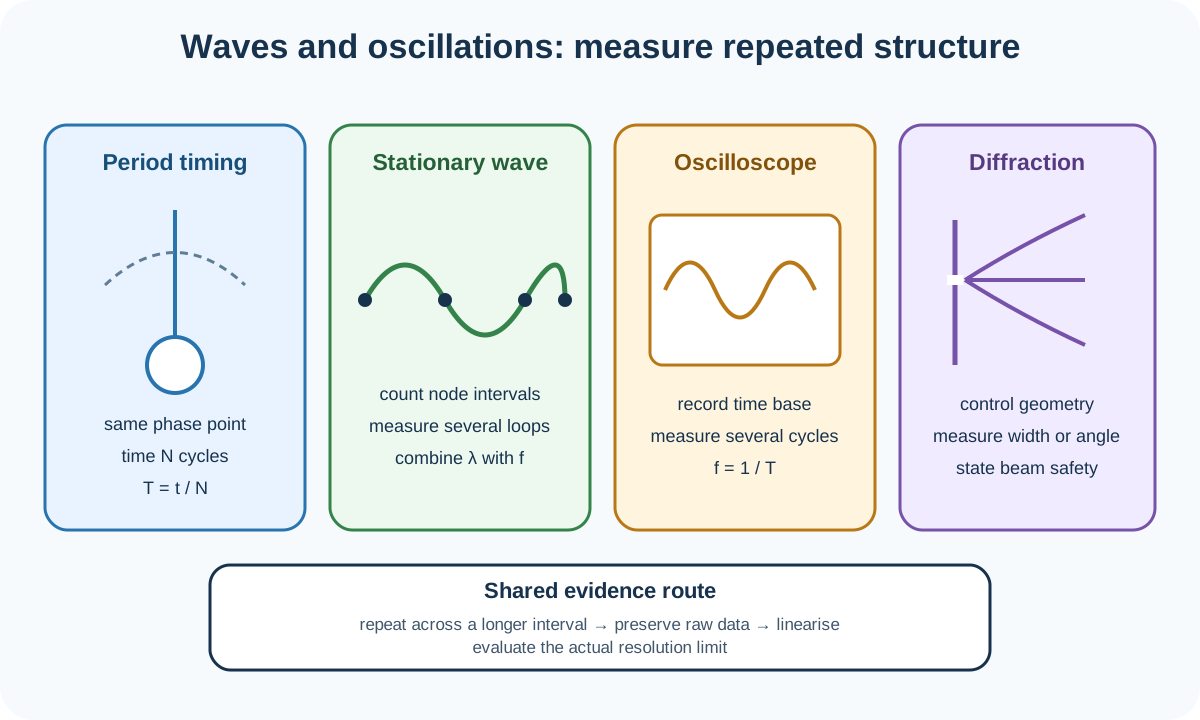
Waves and oscillation experiments are representative contexts for Cambridge International AS and A Level Physics 9702 practical skills. Paper 3 can require candidates to set up unfamiliar apparatus, measure time, length or electrical signals, obtain a useful trend and evaluate an imperfect method. Paper 5 can require a workable plan, oscilloscope or sensor use, linearisation, uncertainty treatment and a conclusion from supplied data.
Official practical boundary
The practical-assessment section requires stopwatch measurement of an oscillating system by timing an appropriate number of consecutive oscillations. It also expects candidates to describe using an oscilloscope to measure voltage, current, time and frequency, and to use suitable sensors or data loggers where relevant.
The syllabus does not prescribe the following as a fixed list of examination experiments. Pendulum timing, stationary waves, signal measurement and diffraction provide varied ways to practise the assessed manipulation, presentation, graph, conclusion and evaluation skills.
Measure a period reliably
Define one complete oscillation and one repeatable phase point before timing. Start and stop as the object passes the same reference in the same direction. Timing opposite-direction crossings would measure half-period intervals while still appearing visually regular.
Time N consecutive oscillations and calculate
T=NtN.
Check this topic from memory
Attempt the matching topic bank before reopening the notes. Use each missed idea to decide what to review next.
Increasing N reduces the fractional contribution of reaction time because the total interval is longer. It does not remove a systematic error in the clock or a changing period. Choose N large enough for a useful interval but not so large that damping or drift materially changes the conditions.
Use a fiducial marker close to the moving object and observe along a fixed line. Keep amplitude within the range assumed by the supplied model, release without a push and repeat the total-time measurement. Use a mean and describe visible variation rather than claiming that every repeat is identical.
For a pendulum-style investigation, measure length between the physical points specified by the model, commonly the suspension point and the centre of the bob. Keep the support rigid and the motion in one vertical plane. A shifting clamp or elliptical path creates a specific limitation that repeats alone cannot correct.
If the given relationship is T=2πL/g, a graph of T2 against L is linear with gradient 4π2/g. The experiment should test the supplied relationship through a range, not calculate g independently from each pair and average away the visible trend.
Measure stationary-wave wavelength
Create a stationary pattern using a driven string, air column or other supplied medium. Adjust frequency, length or tension until nodes and antinodes are stable and clearly defined. Avoid taking readings while the pattern is changing between modes.
For a string segment of length L containing n half-wavelengths,
L=n2λ,λ=n2L.
Measure across several loops rather than one where possible. Dividing a longer measured distance reduces the fractional effect of uncertain node positions. Count intervals between nodes carefully; the number of visible nodes is not automatically the number of half-wavelengths.
Keep tension controlled using the specified hanging load and include the hanger mass if it contributes. Ensure the vibrating length is measured between the effective fixed endpoints. Pulley friction or changing driver behavior can make the actual tension differ from the simple load estimate.
Combine measured wavelength with frequency using v=fλ. If testing how wave speed depends on tension or linear mass density, rearrange the supplied model before choosing graph axes. Do not assume a direct linear plot when the relationship contains a square root.
Use an oscilloscope or data logger
An oscilloscope displays signal variation against time. Set a suitable vertical sensitivity and time base so the trace occupies a useful fraction of the screen without clipping. Count divisions across several cycles, multiply by time per division and divide by the number of cycles to obtain T, then use f=1/T.
State which voltage is connected to the input and where the reference or ground is placed. A stable trigger prevents horizontal drift; it does not change the signal frequency. Calibration settings and probe scale must be included when converting divisions to physical values.
For phase or time delay between two signals, use corresponding points such as rising zero crossings. Measure over several periods when possible. Do not compare a peak on one trace with an unrelated crossing on the other.
A microphone, light sensor, motion sensor or light gate connected to a data logger can reduce reaction-time limitations and capture rapid changes. The sensor still needs calibration, appropriate sampling rate and correct placement. A large digital data set is not automatically accurate if the sensor response or geometry is unsuitable.
Observe diffraction and interference
For diffraction, vary gap width while keeping wavelength and observation geometry controlled, or vary wavelength while maintaining the aperture. Define a measurable outcome such as central-maximum width, angular spread or detector intensity at stated positions rather than relying only on a description that the pattern looks wider.
Measure a screen distance from the aperture plane and mark fringe or maximum positions with a clear reference. For repeated spacings, measure across several intervals and divide by the number of intervals. Keep the aperture, source and screen aligned.
For ripple-tank observations, use a stroboscopic view or image capture if permitted to reduce motion blur. Measure wavelength across several crest separations. Water depth affects wave speed, so keep it controlled unless it is the independent variable.
For light, avoid direct viewing of an intense source and keep the beam below eye level. A laser requires a specific precaution: use a low-power source, terminate the beam and remove reflective objects from the path. "Be careful with the laser" is not a complete risk control.
Tables, graphs and conclusions
Record raw lengths, times, frequencies and scale readings before derived period, squared period, wavelength or speed. Use quantity-unit headings and consistent precision. When logarithms or other derived variables are required, calculate them transparently from the raw columns.
Choose a wide safe range that produces a resolvable dependent change. Plot all observations, use an appropriate best-fit line or curve and identify an anomalous point rather than silently omitting it. Calculate a gradient using points on the line separated by more than half its length.
Relate the gradient or intercept to the requested constant using the rearranged model. Include units and appropriate significant figures. A graph consistent with the model supports it within the tested range and uncertainty; it does not prove universal validity.
Evaluate wave and oscillation methods
Describe the measurement affected and the mechanism. An indistinct node position limits wavelength, a broad bob makes the reference crossing uncertain, falling amplitude may change period under some models, and a sampling rate can be too low for a rapid signal. These are different limitations.
Match the improvement: measure multiple loops for node uncertainty, use a fiducial marker for crossing position, use a rigid release for initial conditions, choose a higher sampling rate for signal resolution or use a stable trigger for trace drift. Repeats reduce random scatter but do not correct a wrong length definition or miscalibrated time base.
Worked application: period graph and gravitational field strength
A pendulum is timed for 20 oscillations at each length, and a graph of T2 against L has best-fit gradient 4.05,s2⋅m−1. From T2=(4π2/g)L, g=4π2/4.05=9.75,m⋅s−2. A worst acceptable line has gradient 4.18,s2⋅m−1, giving gradient uncertainty 0.13,s2⋅m−1, or about 3.2 percent. The percentage uncertainty in g is also about 3.2 percent, so a suitable result is g=(9.8±0.3),m⋅s−2. Timing many oscillations reduces reaction-time fraction, while measuring to the bob's edge instead of its centre would create a length bias that repeats cannot remove.
Common misconceptions and corrections
Timing from one crossing to the next opposite crossing as a full period. Use the same phase point and direction.
Timing one oscillation when many are practical. Increase the total interval and divide by N.
Claiming many cycles remove every timing error. Clock calibration and changing conditions remain.
Starting a pendulum with a push. Use a controlled release.
Measuring pendulum length to an arbitrary edge. Follow the model's defined endpoints.
Allowing an elliptical path. Keep motion in one plane.
Counting visible nodes as half-wavelengths. Count the intervals between adjacent nodes.
Measuring one stationary-wave loop only. Measure across several loops where possible.
Ignoring hanger mass in tension. Include every load component that contributes.
Assuming load weight equals string tension despite pulley friction. Identify the model limitation.
Plotting speed directly against tension without checking the model. Linearise the supplied relationship first.
Reading one oscilloscope cycle when several fit. Measure multiple cycles to reduce reading fraction.
Changing time base and forgetting the new scale. Record the active calibration.
Calling trigger control a frequency control. It stabilises the display.
Comparing unrelated phase points on two traces. Use corresponding features.
Assuming a sensor removes all uncertainty. Calibration, sampling and alignment still matter.
Judging diffraction only by appearance. Define a measurable width, angle or intensity.
Measuring one fringe spacing. Measure across several intervals and divide.
Changing aperture width and screen distance together. Control the observation geometry.
Ignoring water depth in ripple-tank work. It can change wave speed.
Stating only "avoid laser eyes". Terminate a low-power beam below eye level and remove reflections.
Taking gradient points from observations. Use widely separated points on the fitted line.
Saying a straight graph proves the model. It supports the relationship over the tested range.
Assessment guidance
Define the phase point, measured interval and number of oscillations before timing. For stationary waves, state the effective length, mode count, controlled tension and how several loops reduce fractional reading uncertainty. For oscilloscope work, name the connected signal, vertical scale, time base, number of cycles and conversion to period or frequency. Rearrange the supplied model before choosing axes, retain raw readings and use a large gradient triangle. Evaluate a named position, timing, alignment, calibration or sampling mechanism and match it to a realistic modification. Give specific laser, falling-load or electrical precautions where relevant.
Retrieval practice
Plan a pendulum timing investigation, a stationary-string wavelength method and an oscilloscope frequency measurement. Define variables, raw readings, range, repeats and controls; derive one linear graph and its gradient meaning; then identify one random and one systematic limitation, matched improvements and a specific safety control for each relevant setup.
Theory and practical ownership
Theory Topics 7, 8 and 17 explain wave speed, phase, stationary-wave, diffraction, interference and oscillation relationships. This practical note covers how timing, length, electrical traces and pattern positions become controlled data and graph evidence. Practical 1 covers general uncertainty rules, while Practical 6 covers the full cross-context analysis framework.
Cambridge International, AS and A Level Physics 9702 syllabus for examinations in 2025, 2026 and 2027, Practical assessment expectations for Paper 3 Advanced Practical Skills and Paper 5 Planning, Analysis and Evaluation. The named wave and oscillation methods are representative contexts, not a prescribed experiment list.