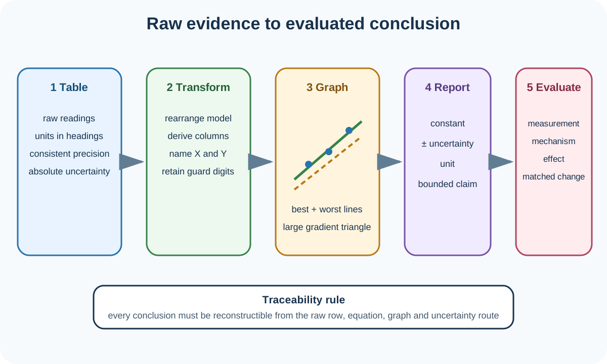
Physics Data Analysis and Evaluation covers the evidence-processing skills assessed across Cambridge International AS and A Level Physics 9702 Papers 3 and 5. Paper 3 turns observations into a table, trend, gradient and bounded conclusion, then asks candidates to diagnose an imperfect method. Paper 5 Question 2 supplies an equation and data from which candidates determine a constant and its uncertainty.
Official analysis boundary
Paper 3 assesses presentation of data, graph layout and plotting, trend lines, gradient and intercept interpretation, conclusions, uncertainty estimates, limitations and improvements. Paper 5 Question 2 is a 15-mark analysis, conclusions and evaluation task covering data analysis, a results table, a graph, a conclusion and uncertainty treatment.
The equation or experimental context may be unfamiliar. Work from the supplied relationship and data. The assessment target is the reasoning chain, not whether the experiment matches a memorised school practical.
Build one traceable results table
Use a single table containing all raw readings and the derived quantities required for analysis. Put the quantity and unit in each heading, for example V/V or t/s. Do not repeat units beside individual entries.
Record a column of raw measurements to a consistent precision when one instrument and method are used. Calculated values should normally have the same number of significant figures as the least precise measured factor, or one more. Retain guard digits during calculation and round the displayed table value coherently.
Check this topic from memory
Attempt the matching topic bank before reopening the notes. Use each missed idea to decide what to review next.
Show absolute uncertainty beside each Paper 5 table value when required. An uncertainty column or value-plus-uncertainty format must make clear which estimate belongs to which quantity.
For logarithms, divide the quantity by its unit before taking the logarithm, such as ln(d/cm). The logarithm itself has no unit. Its decimal places should correspond to the significant figures of the original value: three significant figures commonly lead to three or four decimal places in the logarithm.
Derive the graph from the equation
Rearrange the supplied expression into a linear form before calculating columns. For y=mx+c, plot y against x. For y=axn, plot logy against logx; gradient gives n and intercept gives loga. For y=aekx, plot lny against x; gradient gives k and intercept gives lna.
Write the correspondence explicitly:
Y=mX+c.
Identify Y, X, m and c in terms of the experimental quantities. This determines both the table transformations and the constant-extraction route. A visually straight graph is insufficient if its gradient has not been connected to the requested constant.
Lay out and plot the graph
Label each axis with quantity and unit using the same conventions as table headings. Choose scales so plotted data occupy at least half the available grid in both directions. Use simple scale steps that can be read reliably and place numerical labels regularly. A false origin is acceptable when appropriate, but it must not be treated as numerical zero.
Plot every point to better than 1 mm in Paper 3 expectations. Use a fine cross or small encircled dot. In Paper 5, add error bars in both directions where appropriate, using the absolute uncertainties associated with each point.
Draw a straight best-fit line or suitable curve that represents the overall trend. A best-fit line should balance the scatter along its length rather than join endpoints or pass through every point. Identify a suspected anomaly visibly if excluding it from the fit.
The worst acceptable line is the steepest or shallowest line that remains consistent with all error bars. Draw it as a broken line or label it clearly so it cannot be confused with the best fit.
Determine gradient and intercept
Select two points on the best-fit line separated by more than half its length. These are graph-construction points, not necessarily measured observations. Show the triangle and calculate rise divided by run with axis units.
For a curve, draw a tangent at the requested point and use two well-separated points on that tangent. A chord between nearby data points is not an instantaneous gradient.
Read an intercept directly only when it lies on the plotted axis. If it is off scale or hidden by a false origin, use a point (X,Y) on the fitted line and the gradient:
c=Y−mX.
Then substitute gradient or intercept into the derived expression for the physical constant. Derive its unit from the graph quantities and formula rather than copying a familiar unit from memory.
Treat uncertainty in the final constant
Convert absolute, fractional and percentage uncertainties as needed. For sums or differences, add absolute uncertainties. For products, quotients and powers, add the relevant fractional or percentage contributions using the simple 9702 rules.
For a graph gradient,
Δm=∣mbest−mworst∣.
Use the analogous absolute difference for an intercept. Propagate this estimate through the expression for the required constant. If the constant is inversely proportional to gradient, it has approximately the same percentage uncertainty as the gradient for small uncertainty.
Report the final quantity as value, absolute uncertainty and unit. Round the uncertainty sensibly and round the value to the same decimal place. Do not give a highly precise constant beside a coarse uncertainty.
Draw a bounded conclusion
State what the graph shows and how it addresses the proposed relationship. A straight line supports the chosen linearised form over the tested range within the observed scatter and uncertainties. It does not prove the relationship for all possible values.
For a Paper 3 comparison of two estimates of a constant, calculate percentage difference and compare it with the supplied percentage uncertainty. State whether the difference is within that uncertainty, then conclude whether the data support the relationship by the stated criterion.
Distinguish observation from explanation. "The points curve upward at larger x" is an observation. "Heating changes resistance" is a possible physical explanation that needs support from the apparatus and trend.
Identify limitations precisely
A limitation should identify the affected measurement and the mechanism. Examples include uncertain node position causing wavelength scatter, a broad marker limiting extension readings, source discharge shifting electrical measurements or heat loss making transferred energy smaller than the input estimate.
Prioritise significant effects. A tiny ruler resolution may be less important than a moving clamp. Avoid generic labels such as human error, parallax or friction unless the geometry and consequence are described.
State whether an effect is random, systematic or condition-dependent when that distinction changes the remedy. Repeats and averaging address random variation. Calibration, compensation or redesign address a systematic offset. Alternating measurement order can expose drift.
Suggest matched improvements
Link each improvement directly to a stated limitation. Use a thin fiducial marker and set square for an indistinct extension endpoint, a rigid reference for support movement, a light gate for manual reaction time, insulation and a lid for unwanted thermal transfer, or a high-resistance voltmeter for loading.
Explain how the modification improves the relevant measurement. "Use more accurate equipment" and "repeat more" are incomplete. The improvement must be realistic in a school laboratory and modify the given experiment rather than replacing it with a different one.
Worked application: constant and uncertainty from graph gradients
Data are linearised so that Y=KX. The best-fit line has gradient 2.64,s−1, while the shallowest acceptable line through all error bars has gradient 2.48,s−1. Therefore ΔK=∣2.64−2.48∣=0.16,s−1, a percentage uncertainty of about 6.1 percent. Report K=(2.64±0.16),s−1, or round both coherently to K=(2.6±0.2),s−1. The straight trend supports the supplied proportional form only over the measured range. One high-X point lies outside the apparent scatter; identify it, check its raw reading and apparatus conditions, and do not delete it merely to improve the line.
Common misconceptions and corrections
Creating separate unlinked raw and processed tables. Keep the evidence in one traceable table.
Writing units beside every table entry. Put quantity and unit in the heading.
Changing precision within one raw column arbitrarily. Match the common instrument and method.
Rounding intermediate calculations heavily. Keep guard digits until the reported value.
Giving a logarithm a physical unit. Normalise first; the logarithm is dimensionless.
Using too few logarithm decimal places. Match them to the source value's significant figures.
Choosing graph axes before rearranging the equation. Derive the linear form first.
Using tiny plotted ranges in one corner. Occupy at least half the grid in both directions.
Using awkward scales that are hard to read. Prefer regular simple intervals.
Treating a false origin as zero. Read its actual labelled value.
Drawing thick blobs as points. Use fine marks accurate to better than 1 mm.
Joining points dot to dot. Draw the appropriate trend.
Forcing a best-fit line through every point. Balance scatter along the line.
Deleting an anomaly silently. Identify it and inspect its evidence.
Drawing the worst line outside an error bar. It must remain acceptable for the full set.
Taking gradient points from observations. Use points on the fitted line.
Using a small gradient triangle. Span more than half the line.
Using a chord as a tangent gradient. Draw the tangent at the requested point.
Reading an off-scale intercept as zero. Calculate it from a line point and gradient.
Quoting a constant without deriving its unit. Use graph and equation dimensions.
Using the best-fit gradient alone as uncertainty. Compare best and worst acceptable gradients.
Subtracting signed gradients without taking magnitude. Uncertainty is an absolute difference.
Reporting value and uncertainty at inconsistent decimal places. Round them coherently.
Claiming a straight graph proves a universal law. Bound the conclusion to range and uncertainty.
Naming human error as a limitation. State the measurement mechanism.
Listing an improvement unrelated to the limitation. Match cause and modification explicitly.
Using repeats to correct a systematic bias. Calibrate, compensate or redesign instead.
Assessment guidance
Construct one table with raw and derived values, quantity-unit headings, consistent raw precision and absolute uncertainties where required. Rearrange the equation before calculating transformed columns or selecting axes. Use readable scales, accurate points, appropriate error bars and clearly distinguished best and worst acceptable lines. Take a large gradient triangle from the fitted line, calculate an off-scale intercept algebraically and derive the constant with units. Propagate uncertainty into the final value and round coherently. Conclude only within the tested range, then pair each significant measurement limitation with a realistic improvement that changes its mechanism.
Retrieval practice
Given raw data and a power-law equation, construct the complete table, normalised logarithmic columns and graph plan. Determine best and worst gradients, extract the exponent and its uncertainty, calculate the intercept-derived constant and report it correctly. Then write a bounded conclusion and two limitation-mechanism-improvement chains that distinguish random variation, systematic offset and drift.
Theory and practical ownership
Theory notes explain the subject relationships represented by supplied equations. Practical 1 covers general measurement and uncertainty foundations; Practical 5 covers Paper 5 Question 1 planning. This note covers the cross-context Paper 3 and Paper 5 Question 2 route from raw evidence through table, graph, constant and uncertainty to conclusion and evaluation.
Cambridge International, AS and A Level Physics 9702 syllabus for examinations in 2025, 2026 and 2027, Paper 3 expectations for presentation, graph interpretation, conclusions and evaluation, and Paper 5 Question 2 expectations for data analysis, tables, graphs, conclusions and treatment of uncertainties.