
Cambridge IGCSE Additional Mathematics Notes 7: Straight-Line Graphs

Study guide

Cambridge IGCSE Additional Mathematics notes on line equations, perpendicular bisectors and transformed straight-line relationships.

Cambridge IGCSE Additional Mathematics 0606 Topic 7 covers straight-line equations, parallel and perpendicular conditions, midpoint, length and perpendicular bisectors. It also owns transformation of nonlinear relationships to and from straight-line form so that gradients and intercepts determine unknown constants.
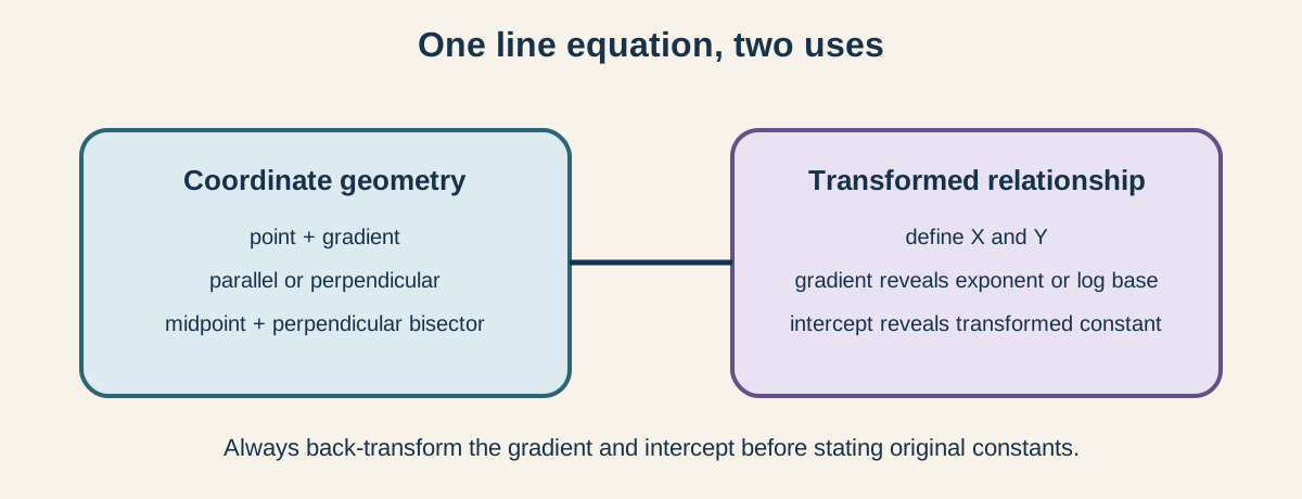
A straight-line topic map connecting coordinate geometry with transformed-variable linearisation

1. Gradient and line equations

For two points, gradient is change in y divided by change in x, using the same subtraction order in numerator and denominator. The form y = mx + c reveals gradient m and y-intercept c. The point-gradient form y - y₁ = m(x - x₁) is efficient when a point and gradient are known.

Other valid forms include ax + by = c and vertical lines x = k. A vertical line has undefined gradient, not zero. A horizontal line has gradient zero and equation y = k.

After forming an equation, substitute every given point and verify its gradient. Simplify into the form requested.

2. Parallel and perpendicular lines

Distinct parallel non-vertical lines have equal gradients. Perpendicular non-vertical, non-horizontal lines have gradients whose product is -1, so one is the negative reciprocal of the other.

Vertical and horizontal lines form the special perpendicular pair. Do not attempt to calculate a negative reciprocal of an undefined gradient.

Geometric conditions must be translated before forming the line. “Parallel to 3x - 2y = 7” first requires rearranging the given line or otherwise identifying its gradient.

3. Midpoint and length

The midpoint of endpoints (x₁, y₁) and (x₂, y₂) averages matching coordinates. The length is the square root of the sum of squared coordinate differences.

Keep an exact square root if later algebra uses the value or exact form is requested. Coordinate differences may be negative, but their squares make length non-negative.

These results help classify shapes, locate centres and construct perpendicular bisectors.

4. Perpendicular bisectors

A perpendicular bisector passes through a segment's midpoint and is perpendicular to the segment. The complete method is:

  1. find the segment gradient;
  2. find the perpendicular gradient;
  3. find the midpoint;
  4. form the line through that midpoint;
  5. verify both conditions.

If the original segment is vertical, its perpendicular bisector is horizontal through the midpoint. If it is horizontal, the bisector is vertical.

5. Why transform a relationship

A nonlinear relationship may become Y = mX + c after defining transformed variables X and Y. A straight-line plot then reveals constants through gradient and intercept.

The axes must be labelled with the transformed quantities, not automatically x and y. The numerical gradient is change in the transformed vertical variable divided by change in the transformed horizontal variable. Interpret m and c through the derived equation before solving for original constants.

6. Power relationships

For y = Axⁿ with positive x and y, take logarithms:

ln y = ln A + n ln x.

Plot Y = ln y against X = ln x. The gradient is n and vertical intercept is ln A, so A = e^(intercept). Common logs work equally if used consistently.

Positivity is required because the logarithms must exist. A straight line supports the power model over the observed domain but does not prove it universally.

7. Exponential relationships

For y = Abˣ with A > 0 and b > 0, take logarithms:

ln y = ln A + x ln b.

Plot ln y against x. The gradient is ln b and the intercept is ln A, hence b = e^(gradient) and A = e^(intercept).

Do not confuse b with ln b or A with ln A. Back-transform both constants.

8. Transforming from a straight line

Cambridge also asks candidates to move from a stated straight-line graph back to an original relationship. If plotting y² against x³ gives gradient A and intercept B, then y² = Ax³ + B. If plotting e^(2y) against x² is straight, define Y = e^(2y) and X = x². If plotting y³ against ln x is straight, then y³ = A ln x + B.

Read the axis labels exactly. An intercept belongs to the transformed dependent quantity, not necessarily to y itself.

9. Data, accuracy and model judgement

Use a ruled best-fit line if the task provides experimental data. Calculate gradient from two well-separated points on the line, not necessarily raw data points. Record transformed units or note when logarithms are dimensionless within the model convention.

Scatter around the line, a restricted data range or systematic curvature limits the model. Interpolation is generally safer than extrapolation.

Worked example: recover a power model

Measurements are believed to follow y = Axⁿ. A graph of ln y against ln x is a straight line through transformed points (0.4, 1.1) and (1.6, 3.5), with vertical intercept 0.3. Its gradient is (3.5 - 1.1)/(1.6 - 0.4) = 2.4/1.2 = 2, so n = 2. The intercept is ln A = 0.3, hence A = e^0.3 ≈ 1.35. The model is therefore y ≈ 1.35x². Substitution of either transformed point checks consistency: when ln x = 0.4, predicted ln y = 0.3 + 2(0.4) = 1.1. Reading A as 0.3 would confuse the logarithm of the constant with the constant itself.

Common misconceptions and how to correct them

  • Subtracting coordinates in opposite orders. Use the same point order in both changes.
  • Calling a vertical gradient zero. Vertical gradient is undefined.
  • Using a negative reciprocal for parallel lines. Parallel gradients are equal.
  • Ignoring the vertical-horizontal perpendicular case. Handle it without reciprocal arithmetic.
  • Using endpoint differences for a midpoint. Average corresponding coordinates.
  • Checking only midpoint for a perpendicular bisector. Verify perpendicularity too.
  • Plotting y against x for every transformed model. Define the required X and Y axes.
  • Reading n from an intercept in a power model. n is the log-log gradient.
  • Reading A as ln A. Exponentiate the intercept.
  • Reading b as the exponential-plot gradient. The gradient is ln b.
  • Forgetting log positivity restrictions. Power and exponential log transforms require valid positive quantities.
  • Claiming a straight plot proves a model everywhere. It supports it only over tested data.

Assessment guidance

Show gradient calculation with consistent coordinate order and form each line through a known point. For parallel or perpendicular questions, state the gradient condition explicitly. A perpendicular-bisector solution must contain midpoint and perpendicular-gradient evidence. In transformation questions, derive the straight-line equation, define transformed axes and identify which expression equals the gradient and intercept. Back-transform logarithmic constants before reporting the original model. When data are supplied, use suitable widely separated best-fit-line points and comment cautiously on fit and extrapolation. Correct algebra with incorrectly labelled axes does not establish the requested transformed relationship.

Retrieval practice

Form equations of four lines, including vertical, parallel and perpendicular cases. Calculate a length, midpoint and perpendicular bisector. Transform power and exponential relationships to straight-line form, identify axes, gradient and intercept, then recover constants from sample graph values. Reverse three stated transformed plots into original equations and explain one limitation of extrapolating each model.

Return to the Additional Mathematics hub.

Official source

Cambridge International, Additional Mathematics 0606 syllabus for examinations in 2025, 2026 and 2027.

Check this topic from memory

Attempt the matching topic bank before reopening the notes. Use each missed idea to decide what to review next.

Start the topic quiz

Sources

  1. Cambridge IGCSE Additional Mathematics 0606 syllabus for 2025-2027