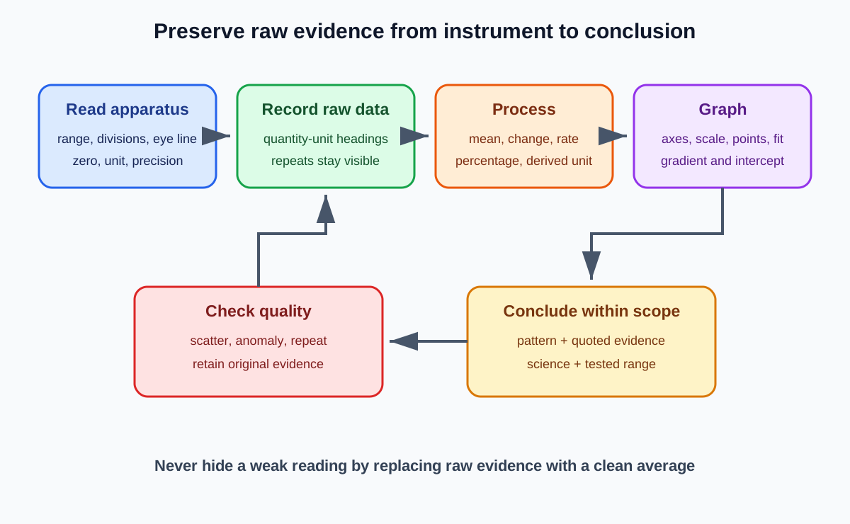
Cambridge IGCSE Co-ordinated Sciences 0654 requires candidates to read analogue and digital apparatus, record observations systematically, process evidence, present it graphically and interpret patterns. Good presentation is part of the experiment: it preserves enough raw evidence for another reader to inspect every calculation and conclusion.
Match apparatus to quantity and range
First identify the quantity: length, volume, mass, temperature, time, force, current, potential difference or another derived quantity.
Then check whether the instrument covers the expected range. An instrument with a smaller capacity may provide finer divisions for a small measurement, but it must still contain or reach the quantity safely.
Do not select an instrument merely because it appears sophisticated. Its scale and operating method must fit the task.
Use resolution to justify precision
Resolution is the smallest change that an instrument can display or that can be distinguished on its scale.
Smaller scale divisions can support a more precise reading, provided the apparatus is used correctly. A choice should be justified with this feature rather than the unsupported phrase “more accurate”.
Do not write decimal places that the scale cannot support. Extra digits create an appearance of certainty without new information.
Decode an analogue scale before reading
Identify two labelled marks, find their numerical difference and divide by the number of intervals between them. That gives the value of one smallest division.
Only then locate the pointer, liquid level or other indicator. The syllabus may require a reading to the nearest half-scale division.
Count intervals rather than lines: five marked lines can enclose four intervals.
Read without parallax
Place the line of sight perpendicular to the scale and level with the indicator. For an ordinary liquid meniscus, read the specified part consistently.
Viewing from above or below can shift the apparent alignment and introduce a reading error.
A mirror scale or fixed pointer can help establish the correct line of sight when supplied.
Record digital readings as displayed
A digital instrument gives a direct displayed value, but it still has limited resolution and range.
Record the displayed precision unless the question instructs a conversion. Do not append unsupported zeroes or discard a displayed final digit without reason.
Check the unit, selected range and any sign or multiplier shown on the instrument.
Check and correct zero error
Check this topic from memory
Attempt the matching topic bank before reopening the notes. Use each missed idea to decide what to review next.
An instrument should indicate zero when the measured quantity is zero under its operating conditions.
If a zero offset exists and a correction is required, apply it consistently to all relevant readings. A positive offset must be subtracted; a negative offset requires the corresponding correction in the other direction.
State the raw reading and correction logic so the processed value can be audited.
Use consistent units before calculation
Units belong to quantities, not as decorative labels. Record the unit shown, then convert only when a formula or comparison requires consistency.
For example, metres and seconds are needed for a speed in metres per second. Cubic centimetres may be converted where another quantity is expressed in cubic metres.
Write the conversion explicitly instead of changing a number silently.
Prepare a table before collecting evidence
Place the independent variable in the first column, followed by raw dependent-variable readings and then processed quantities.
Use one value per cell. Give each heading as quantity and unit, such as time / s or temperature / °C.
Planning the table first reduces omitted readings and reveals whether repeats or calculations have been properly designed.
Preserve raw measurements
Keep every repeat before presenting a mean, rate, difference, ratio or percentage.
Raw evidence shows scatter and makes anomaly decisions checkable. A processed value alone hides the quality of its inputs.
If an instructed correction is applied, retain enough information to show how the corrected result arose.
Record precision consistently
Measurements made with the same instrument under the same conditions should normally use the same decimal places within a column.
Calculated values should use a sensible precision supported by the input readings. Copying all calculator digits does not improve validity.
Qualitative observations also need precision of language: colour, state, precipitate, gas or structural feature rather than only “changed”.
Calculate a representative mean
Add the accepted repeat values and divide by the number included. Show which values are included if an anomaly is excluded.
A mean can reduce the influence of random variation. It cannot correct a consistent calibration offset or an uncontrolled method.
Keep units and round in line with the original measurement quality.
Calculate differences, rates and percentages
A change is final value minus initial value. Preserve its sign when direction matters.
A rate is change divided by time. Reciprocal time is a comparative rate only when every trial reaches the same fixed endpoint.
Percentage change is change divided by initial value, multiplied by 100. It supports comparison when starting values differ, but the initial value cannot be zero.
Choose a display that matches the variables
Use a line or scatter graph when both variables are numerical and continuous and intermediate values are meaningful.
Use a bar chart for separate categories or discrete groups. Bars should have equal width and gaps. A histogram represents grouped continuous data, so adjacent class bars touch.
Do not choose a graph type merely because it is familiar. Match the display to the data structure.
Put variables on the correct axes
The independent variable normally goes on the horizontal x-axis and the dependent variable on the vertical y-axis unless instructions specify otherwise.
Label each axis with quantity and unit. A symbol alone may be insufficient if it is not clearly defined.
The plotted relationship should correspond exactly to the table columns or processed quantities requested.
Select a clear numerical scale
Choose simple intervals based on 1, 2 or 5 units per convenient grid interval. Use more than half the available grid in both directions.
Axes need not begin at zero unless the context or requested interpretation requires it. Show any non-zero start clearly.
Avoid awkward scales that make accurate plotting or reading unnecessarily difficult.
Plot points precisely
Plot each coordinate as a small cross or another precise accepted mark. Large blobs obscure the value.
Recheck the table row, axis scale and coordinate order when a point appears far from the pattern.
Do not move a plotted point merely to make the graph smoother.
Draw an evidence-based fit
Use a straight best-fit line when the data support a linear relationship, or a smooth curve when the relationship changes continuously.
A fit represents the overall pattern and should not join every point dot to dot. With scatter, aim for a reasonable balance around the line.
Do not force the fit through the origin unless evidence, theory or instructions justify that constraint.
Calculate gradient from the fitted line
Choose two well-separated points on the best-fit line, not necessarily raw plotted points. Draw a large triangle and calculate vertical change divided by horizontal change.
Include the sign and units, derived from the y-axis unit divided by the x-axis unit.
Using nearby points magnifies reading uncertainty and can produce an unstable gradient.
Interpret an intercept
An intercept is where the fitted relation crosses an axis. Its unit matches the quantity represented on that axis.
An intercept may represent an initial value, background effect or systematic offset, depending on the experiment.
Do not assign a physical meaning without linking it to the variables and method.
Separate interpolation from extrapolation
Interpolation estimates a value within the measured data range. Extrapolation extends the fitted relationship beyond the tested range.
Extrapolation is less secure because the relationship may change outside the observations. State this limitation when it matters.
Show construction lines if the question asks for a value read from the graph.
Identify an anomaly from the pattern
An anomalous value lies unexpectedly outside the general pattern or differs strongly from other repeats under the same condition.
Check transcription, scale reading, setup changes and procedural records. Repeat the condition where feasible while retaining the original value.
An unexpected result is not automatically an error, especially in biological data where genuine variation is common.
Compare values within experimental accuracy
The syllabus allows candidates to judge whether results are equal within limits of experimental accuracy, assumed as plus or minus 10 percent at this level.
Use a quantitative comparison rather than visual impression. Preserve the actual values and explain the basis of the judgement.
This instruction does not make every difference below 10 percent scientifically meaningless in all contexts.
Link graph evidence to the conclusion
Describe direction, shape, turning point, plateau or proportionality only when the evidence supports it. Quote representative values, a gradient or another processed feature.
Explain the pattern with relevant Biology, Chemistry or Physics only after stating what the data show.
Keep the claim within the measured range and acknowledge scatter or uncertainty where important.
Worked application: process a gas-volume investigation
A reaction produces gas volumes of 31, 30 and 32 cm³ after 40 s at one concentration. Record the three raw readings in separate columns and calculate a mean of 31 cm³. The mean production rate over that interval is 31 divided by 40, or 0.775 cm³ per second, reported to suitable precision. Plot concentration on the x-axis and mean rate on the y-axis. If a repeat were 12 cm³, first check for leakage, a blocked connection or transcription error and repeat that concentration. Preserve the 12 cm³ result rather than deleting it silently before fitting the trend.
Common misconceptions and corrections
Selecting apparatus without checking range. It must contain or reach the expected value.
Calling smaller divisions automatically more accurate. They support precision, while technique and bias affect accuracy.
Counting scale lines instead of intervals. Divide by the spaces between marks.
Reading a meniscus from above. Align the eye to reduce parallax.
Adding decimal places to a digital display. Record only supported precision.
Ignoring the instrument unit or range setting. Both affect the reading.
Repeating readings without checking zero error. Repeats preserve a systematic offset.
Applying a zero correction in the wrong direction. Reverse the offset.
Mixing units inside one calculation. Convert explicitly first.
Putting units in every table cell. Put them in headings.
Writing only the unit in a heading. Include quantity and unit.
Putting the dependent variable first by default. Independent normally comes first.
Replacing repeats with only a mean. Preserve raw evidence.
Using inconsistent decimal places in one instrument column. Match resolution.
Copying every calculator digit. Use justified precision.
Recording “positive” instead of an observation. Describe the visible result.
Calculating a mean without showing included values. Make anomaly handling auditable.
Saying a mean removes systematic error. It reduces random influence only.
Using reciprocal time for changing endpoints. The endpoint must be fixed.
Ignoring the sign of a change. Direction can matter.
Using a line graph for named categories. Use a bar chart.
Drawing touching category bars. Bar-chart bars have gaps.
Drawing histogram bars with gaps. Continuous intervals touch.
Putting the dependent variable on x without instruction. Independent normally goes there.
Using less than half the grid. Expand the scale.
Choosing awkward intervals such as 3 or 7. Prefer 1, 2 or 5 based steps.
Plotting large blobs. Use precise small marks.
Joining every point dot to dot. Use an appropriate fit.
Forcing the line through zero. Require evidence or justification.
Taking gradient from adjacent raw points. Use a large triangle on the fit.
Omitting gradient units. Derive y-unit divided by x-unit.
Giving an intercept a meaning without context. Link it to the method.
Calling an in-range estimate extrapolation. It is interpolation.
Treating extrapolation as certain. The relation may change.
Deleting an anomaly silently. Retain, investigate and repeat.
Calling every unusual biological result an error. Genuine variation occurs.
Applying the 10 percent statement as universal rounding. Use it for the stated equality judgement.
Writing a conclusion with no values. Cite evidence.
Claiming causation from an uncontrolled graph. Evaluate the design.
Generalising beyond the measured range. Scope the claim.
Assessment guidance
Decode every scale before reading and use only supported precision. Tables need independent variable first, quantity-unit headings, raw repeats, consistent decimal places and separate processing. For graphs, choose the correct display, label both axes, use more than half the grid, plot precisely and fit the evidence. Calculate gradient from a large triangle on the fit with units. Distinguish interpolation from riskier extrapolation. Anomaly responses should identify, check, repeat and preserve evidence. Conclusions need the numerical pattern and a scope-limited scientific explanation.
Retrieval practice
Decode ten analogue and digital scales, including two zero errors. Build tables that preserve repeats before means, rates and percentages. Choose displays for continuous, categorical and grouped data. Plot three datasets with 1, 2 or 5 based scales, calculate gradients and intercepts with units, classify interpolations and extrapolations, and write defensible anomaly decisions and evidence-linked conclusions.
Topic ownership
This note owns the official AO3 requirements for readings, precision, zero correction, systematic recording, processing, graphical presentation, gradient, intercept, interpolation, extrapolation, conclusions and anomaly handling. Practical 2 owns complete planning and evaluation logic. Practicals 4 to 7 own context-specific measurement choices, while practical 8 consolidates apparatus and improvements.