Cambridge IGCSE Statistics 3: Frequency distributions

Cambridge IGCSE Statistics 0479 Topic 3 develops grouped and ungrouped frequency distributions, class notation, histograms, frequency polygons and cumulative frequency representations. The central principle is that a display must preserve the meaning of frequency even when class widths differ.

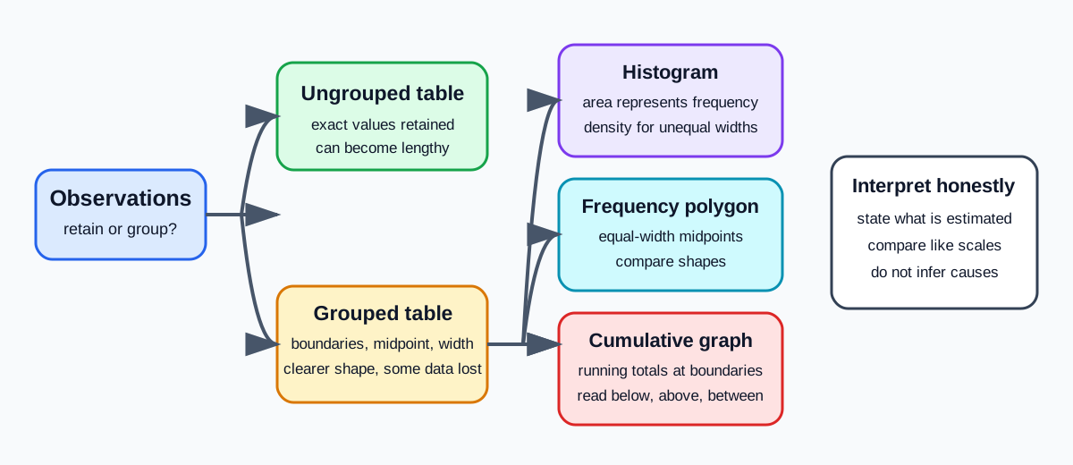
1. Ungrouped and grouped frequency distributions

An ungrouped frequency distribution records every distinct value and its frequency. It preserves exact values and supports exact calculations, but a long table can conceal the overall pattern.

A grouped distribution combines values into non-overlapping classes, such as 30 ≤ x < 40. Grouping makes shape, concentration and spread easier to see. Its cost is information loss: the original values within each class are unknown, so later calculations based on class midpoints are estimates.

Classes must cover the relevant range without gaps or overlaps. State the convention clearly. The class 30 ≤ x < 40 includes 30 but excludes 40, which enters the next class.

2. Class limits and boundaries

For discrete data, class limits are the smallest and largest recorded values assigned to a class. If ages in completed years are grouped as 10 to 14, the lower and upper class limits are 10 and 14. Assuming measurement to the nearest year, the corresponding continuous class boundaries are 9.5 and 14.5.

For continuous data, classes are defined by boundaries directly. A mass class 50 ≤ m < 60 has boundaries 50 and 60. There is no artificial gap between it and 60 ≤ m < 70.

The class midpoint is (lower boundary + upper boundary) ÷ 2.

The class width is upper boundary minus lower boundary. Use boundaries, not displayed integer limits, when determining histogram widths.

3. Histograms and frequency density

A histogram represents continuous grouped data with touching rectangles. The area of each rectangle represents frequency. With equal class widths, frequency and frequency density produce the same relative pattern, but with unequal widths the vertical axis must be frequency density:

frequency density = frequency ÷ class width

Therefore:

frequency = frequency density × class width

Label both axes with the variable and units. The horizontal scale follows class boundaries. The vertical scale is frequency density, including compound units when appropriate, such as people per minute.

A taller bar does not necessarily contain more observations. Compare areas when widths differ. To find a frequency from a published histogram, read the density and multiply by the relevant width. If the vertical scale is absent but one class frequency is known, use that class to establish the scale factor.