Cambridge IGCSE Statistics 8: Probability distributions

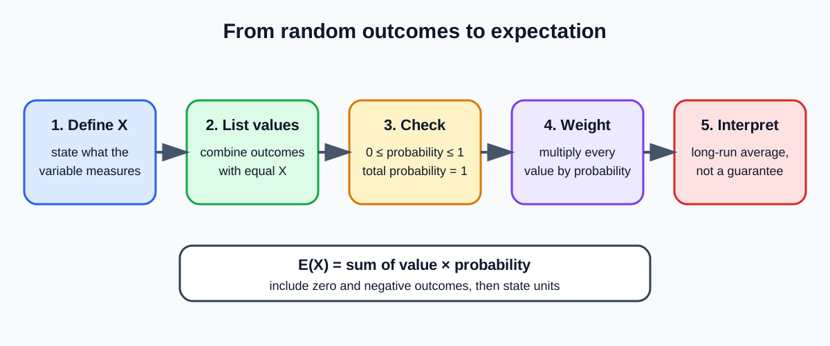
Cambridge IGCSE Statistics 0479 Topic 8 requires learners to construct probability distributions for simple situations and calculate or use expectation. A distribution connects every possible value of a random variable to its probability, and its probabilities must total 1.

1. Random variables and possible values

A random variable assigns a numerical value to each outcome of a random process. It may count successes, record a score, or represent a monetary gain or loss. Use a clear symbol such as X and define what it measures.

Distinct outcomes can produce the same X-value. If two different spinner results both give a score of 3, combine their probabilities in the distribution row for X = 3. The distribution lists values, not necessarily every underlying outcome separately.

The values must be mutually exclusive and collectively exhaustive: exactly one listed value occurs in each trial, and no possible value is omitted.

2. Constructing a probability table

A discrete probability table normally has one row for x and one for P$X = x$. Generate the sample space systematically using a list, grid or tree, calculate the probability attached to each value, then combine equal values.

Check two conditions:

• every probability lies from 0 to 1 inclusive
• the sum of all probabilities equals 1

If a probability is represented by a parameter, use the total of 1 to solve it. Then verify the resulting values remain valid. An algebraic solution that makes a probability negative is not acceptable.

3. Deriving event probabilities from a distribution

Once the table is complete, add the probabilities for values satisfying the event. For example, P(X at least 2) includes X = 2 and every larger listed value. P(X below 2) excludes 2. Translate inequalities carefully before summing.

The complement can shorten work. P(X at least 1) equals 1 - P$X = 0$ when zero is the only way to have no successes.

A distribution can use fractions, decimals or percentages, but one consistent exact form makes checking easier.

4. Expectation

The expectation or expected value is a probability-weighted mean:

E(X) = sum of [x × P$X = x$]

Create a product row, sum it, and retain signs for losses or negative scores. Expectation has the same units as X. It need not be a possible outcome: an expected 1.6 successes describes a long-run average, not a result obtainable in one integer-valued trial.

Over many comparable independent repetitions, total expected value is:

number of trials × expectation per trial

This is a long-run model, not a guarantee of the realised total.

5. Gains, costs and fair games

Define net gain consistently. If a player pays an entry fee, subtract it from every prize outcome or calculate expected prize and then subtract the fee once per play.

A game is fair in the expectation sense when expected net gain is zero. Positive expected net gain favours the player in the long run; negative expected net gain favours the organiser. Fair expectation does not mean equal chances of winning and losing, and it does not remove short-term risk.

To find a fair fee, set expected net gain to zero. To find a missing prize, place it in the relevant value-probability product and solve the expectation equation.

6. Transforming expectation

If every outcome is changed by a linear rule Y = a + bX, then:

E(Y) = a + bE(X)

This follows because the same fixed addition affects every outcome, while multiplication scales every value. It can simplify problems involving a fixed bonus, tax, conversion factor or entry cost.

Do not apply a non-linear operation in the same way. In general, the expected value of X squared is not the square of E(X).

7. Interpreting decisions responsibly

Expectation compares long-run averages. A choice with higher expectation can still have a larger chance of a severe loss. The Topic 8 syllabus requires expectation, not a full risk-analysis framework, but good interpretation distinguishes expected return from certainty and acknowledges the time horizon.

Probability assumptions also matter. If the distribution was built from an unfair spinner, changing population or uncertain estimate, its expectation is only as reliable as those probabilities.

Worked example: prize game and fair entry fee

A game pays $12 with probability 0.1, $4 with probability 0.3 and $0 with probability 0.6. The expected prize is 12 × 0.1 + 4 × 0.3 + 0 × 0.6 = $2.40. Therefore $2.40 is the fair entry fee in the expectation sense. If the actual fee is $3, define net gains as $9, $1 and -$3. Their expectation is 9 × 0.1 + 1 × 0.3 - 3 × 0.6 = -$0.60 per play. Across 200 comparable plays, the expected total player gain is -$120, but an individual run can differ substantially. The calculation predicts a long-run average, not a guaranteed loss on each play.

Common misconceptions and how to correct them

• Listing outcomes but not random-variable values. Combine outcomes that produce the same value.
• Omitting a possible value with small probability. The table must be exhaustive.
• Allowing overlapping value categories. Exactly one listed value must occur.
• Accepting probabilities that do not total 1. Use the sum as a validity check.
• Solving a parameter but not checking its range. Every probability must lie from 0 to 1.
• Treating “at least 2” as only X = 2. Include all larger allowed values.
• Averaging listed x-values without probabilities. Expectation is weighted.
• Forgetting negative signs for losses. Use net values consistently.
• Assuming expectation must be an obtainable outcome. It is a long-run mean.
• Calling expectation the most likely value. The mode is the most probable value.
• Claiming expected value will occur in one trial. It is not a prediction of one result.
• Multiplying only prizes by probability but ignoring zero or loss outcomes. Include all values.
• Subtracting an entry fee only from winning outcomes. It is paid on every play.
• Calling equal win and loss probabilities a fair game. Fairness here requires zero expected net gain.
• Treating positive expectation as risk-free. Outcomes still vary.
• Assuming E(X²) equals [E(X)]². Linear rules transfer directly; non-linear ones generally do not.

Assessment guidance

Define the random variable and build the sample space systematically before combining equal values. Display a complete table and show that probabilities sum to 1, especially after solving an unknown parameter. In expectation calculations, include a visible xP$X = x$ row or equivalent working, retain negative gains and state units. Translate “at least”, “more than” and “at most” precisely. For games, distinguish prize from net gain and subtract fees consistently. Interpret expectation as a long-run average, not a guaranteed single outcome, and state what positive, zero or negative expected net gain means in context.

Retrieval practice

Build distributions from a two-coin experiment, a spinner sum and a simple prize game. Solve one missing probability and reject an invalid parameter value. Calculate probabilities of inequality events, expectations and expected totals over repeated trials. Determine a fair entry fee and a missing prize, then explain why the expected value can differ from both the most likely outcome and any possible single result.

Return to the Statistics hub.