

Cambridge IGCSE Statistics 12: Time series

Study guideUpdated 27 Aug 2026

Cambridge IGCSE Statistics 0479 notes on time series.

Cambridge IGCSE Statistics 0479 Topic 12 covers time-series graphs, moving averages and centring, trend, seasonal components, prediction, and the assumptions and limitations behind forecasts.
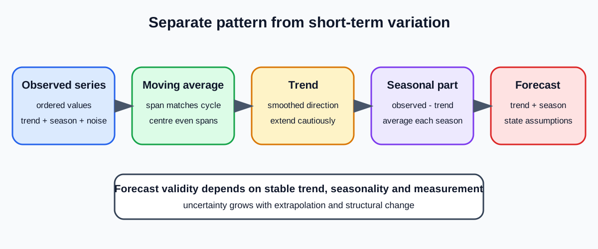
A decomposition workflow from observed time-series data through centred moving averages and seasonal components to a forecast

1. Time-series structure

A time series records one variable in chronological order, usually at equal intervals. Its observed movement may contain:

  • trend, the longer-term direction
  • seasonal variation, a pattern repeating at a fixed known period
  • irregular variation, unpredictable short-term movement

A rise followed by a fall is not automatically seasonal. Seasonality requires repetition at corresponding positions in successive cycles.

2. Plotting a time-series graph

Put time on the horizontal axis and the measured variable, with units, vertically. Use a consistent time scale and plot in chronological order. Joining successive points is appropriate because sequence is part of the data, unlike a scatter diagram.

Choose a scale that shows variation without distorting it. If a vertical-axis break is used, make it explicit. Label years, quarters or months carefully so observations are not shifted by one period.

The raw graph helps identify overall direction, seasonal repetition, turning points and unusual values, but short-term fluctuations can obscure trend.

3. Moving averages

A moving average smooths irregular and seasonal variation by averaging consecutive observations. Choose a span matching the seasonal cycle: four quarters, twelve months, or another stated period.

For a four-point moving average, average observations 1 to 4, then 2 to 5, then 3 to 6, continuing one period at a time. Every window must contain exactly four values.

Moving averages lose observations at both ends because complete windows are unavailable there. This is a structural consequence, not a calculation mistake.

4. Positioning and centring

An odd-span moving average lies naturally at its middle time point. A three-point average of periods 1 to 3 is plotted at period 2.

An even-span average lies between two time points. A four-point average for periods 1 to 4 lies between periods 2 and 3, so it does not align with an original observation. Centre it by averaging two adjacent four-point moving averages. The resulting centred moving average aligns with the shared intervening period.

Centre only when alignment requires it. Do not centre an already aligned odd-span series automatically.

5. Trend

Centred moving averages estimate the trend-cycle component by smoothing seasonal effects. Plot them at correct time positions and draw a trend line by eye through their central pattern when requested.

A trend line should reflect the moving-average values rather than chase each raw observation. It can be linear over the observed interval even if long-term behaviour may eventually change.

Read trend values with sensible graphical precision. A fitted trend is an estimate, not an exact underlying law.

6. Seasonal components

In the additive model used for these calculations:

seasonal variation = observed value - trend value

Seasonal variation is positive when the observation lies above trend and negative when it lies below. Obtain values from a table of observations and moving averages or read observations and trend values from a graph.

Group variations by corresponding season, such as all first quarters, and average them to estimate each seasonal component. The components across one complete cycle should total approximately zero. If rounding or sampling leaves a small discrepancy, follow the correction method requested.

A seasonal component of +8 means that season tends to lie 8 units above trend, not that it grows by 8%.

7. Forecasting

For an additive forecast:

forecast = trend prediction + seasonal component

First extend or evaluate the trend for the required period, then add the matching season's component. Keep season labels aligned: a Quarter 3 component must be used for Quarter 3.

If a question supplies a trend equation, substitute the correct coded time. If it supplies a graph, read the trend value before applying seasonality.

8. Assumptions and limitations

Forecasting assumes that the estimated trend continues and the seasonal pattern remains sufficiently stable. It also assumes comparable measurement definitions and intervals.

Predictions become less reliable farther beyond observed data. Structural breaks, policy changes, new competitors, unusual weather, changing population, capacity limits and one-off shocks can invalidate historical patterns. A small data set may provide weak seasonal estimates.

The model does not attach certainty to a forecast. State both the numerical prediction and the assumptions on which it depends.

Worked example: centred averages and seasonal forecast

Quarterly sales are 80, 96, 110, 94, 88, 104, 122 and 102. The first two four-quarter moving averages are (80 + 96 + 110 + 94) ÷ 4 = 95 and (96 + 110 + 94 + 88) ÷ 4 = 97. Their centred average is 96, aligned with Quarter 3 of the first year. Since the observed value there is 110, its seasonal variation is 110 - 96 = +14. Suppose averaging all Quarter 3 variations gives a seasonal component of +13 and the trend forecast for a future Quarter 3 is 118. The additive forecast is 118 + 13 = 131, assuming trend and seasonality persist.

Common misconceptions and how to correct them

  • Plotting time in arbitrary order. Preserve chronology.
  • Treating a time-series graph like an unjoined scatter plot. Sequence links adjacent observations.
  • Calling any fluctuation seasonal. Look for fixed-period repetition.
  • Choosing a moving-average span unrelated to the cycle. Match the seasonal period.
  • Changing the number of values between windows. Keep the span fixed.
  • Moving the window by its full width. Shift one period at a time.
  • Expecting moving averages at both endpoints. Complete windows are unavailable there.
  • Plotting an even-span average at an original time point. It lies between points before centring.
  • Centring an odd-span average unnecessarily. It already has a middle observation.
  • Averaging non-adjacent moving averages to centre. Use adjacent values.
  • Drawing trend through every raw fluctuation. Follow the smoothed central direction.
  • Calculating seasonal variation as trend minus observed. For the additive model, use observed minus trend.
  • Treating a seasonal component as a percentage. It has the original additive units.
  • Mixing seasonal labels across cycles. Average corresponding seasons only.
  • Subtracting seasonality when forecasting regardless of sign. Add the signed component.
  • Using the wrong coded time in a trend equation. Map time labels explicitly.
  • Presenting an extrapolated forecast as certain. State stability assumptions and horizon limits.

Assessment guidance

Label time and measurement axes with units and keep periods equally spaced. In moving-average work, show every window and divisor, then place values at their correct temporal positions. Explain why even spans need centring and show adjacent-average calculations. Derive seasonal variations consistently as observed minus trend, average corresponding seasons and check their cycle total is near zero. For a forecast, state the trend value, matching seasonal component and signed addition. Evaluation should name the extrapolation horizon and concrete reasons trend or seasonality might change, rather than merely saying the prediction may be inaccurate.

Retrieval practice

Plot a quarterly time series and identify plausible trend, seasonal and irregular features. Calculate three-point and four-point moving averages, centre the even-span series and plot it correctly. Derive seasonal variations from both a table and graph, average them into components, check their total, construct forecasts for four seasons, and explain how structural change and increasing forecast horizon affect reliability.

Return to the Statistics hub.

Check this topic from memory

Attempt the matching topic bank before reopening the notes. Use each missed idea to decide what to review next.

Start the topic quiz

Sources

  1. Cambridge IGCSE Statistics 0479 specification