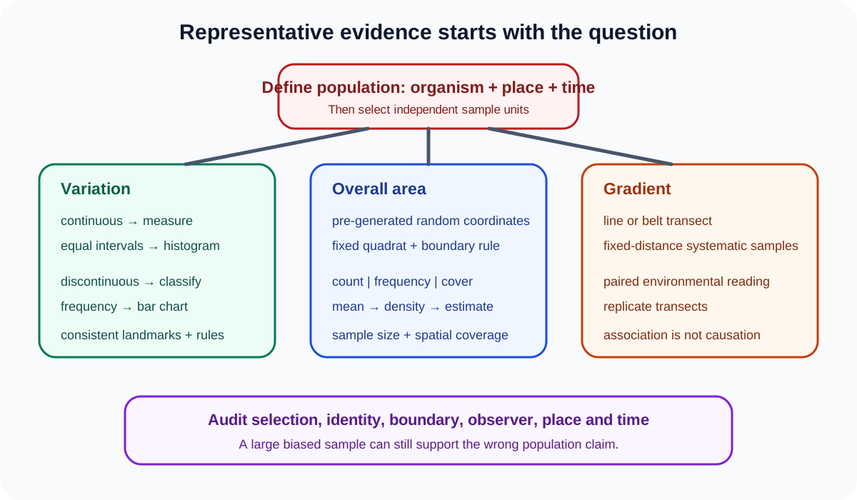
Cambridge IGCSE Biology 0610 and 0970 require investigation of continuous and discontinuous variation and representative, bias-avoiding sampling with attention to sample size and simple random sampling. Ecological questions may supply unfamiliar organisms, apparatus or environmental gradients, so the method must be justified from the evidence needed.
Define the target population
The target population is the complete group about which a conclusion is intended. A sample is the subset measured.
Define the population by organism, place and time. "Leaves" is vague; "mature leaves on ten plants along the eastern boundary on the sampling date" is reproducible.
A sample can be large yet unrepresentative if it comes from one convenient corner. Representativeness depends on selection method as well as number.
Investigate continuous variation
Continuous variation has a range of numerical values with intermediates, such as leaf length or human height. Choose clear measurement landmarks, suitable apparatus and consistent precision.
Measure enough independent individuals to display the distribution. Do not repeatedly measure one leaf and call those values a population sample.
Record raw values, calculate a mean and range where useful, and group values into equal continuous intervals for a histogram. Histogram bars touch because adjacent classes share a continuous scale.
Choose intervals that reveal the distribution without producing one broad bar or many nearly empty bars. State class boundaries clearly so every value belongs once.
Investigate discontinuous variation
Discontinuous variation forms distinct categories with no intermediate values, such as ABO blood group or the ability to roll the tongue in the common syllabus examples.
Define categories before counting and classify every individual using the same rule. Display frequencies in a bar chart with separated equal-width bars.
Do not measure a categorical trait with an invented continuous scale. Some real traits are harder to classify than textbook examples, so acknowledge ambiguous cases and use an agreed rule.
Human variation investigations require consent, privacy and non-sensitive traits. Use anonymous codes and avoid claims about health, intelligence or personal worth.
Use simple random sampling
Simple random sampling gives every eligible location or individual an equal selection chance. For an area, place two perpendicular coordinate axes along its edges and use random-number pairs to choose positions.
Place a quadrat using a stated corner or centre at each coordinate. Generate coordinates before looking at vegetation, so attractive or convenient patches do not influence selection.
Check this topic from memory
Attempt the matching topic bank before reopening the notes. Use each missed idea to decide what to review next.
If a coordinate is inaccessible, use a predeclared rule such as generating a replacement rather than choosing the nearest easy location.
Random does not mean throwing a quadrat casually. Throws may cluster near the sampler, avoid obstacles and differ in strength or direction.
Select a quadrat measure
Count individuals when organisms are separate and identifiable. Frequency records presence or absence in quadrats. Percentage cover estimates the proportion of ground occupied and suits spreading or overlapping plants.
State the abundance measure before sampling. Counts, frequency and cover answer different questions and should not be combined as if they were the same unit.
Use a gridded quadrat or defined cover categories to make percentage estimates consistent. Train observers with the same reference examples.
Apply boundary and identity rules
An organism crossing a quadrat edge must be treated by a predefined inclusion rule, such as count those touching the top and left boundaries but not bottom and right. Apply it at every location.
For clonal or mat-forming plants, defining an individual may be difficult. Percentage cover can be more defensible than count.
Use an identification key or reference and record uncertain specimens separately. Changing identification decisions after seeing the results introduces bias.
Choose a suitable sample size
More independent random quadrats generally reduce the influence of local patchiness and improve precision. The number needed depends on area size, organism distribution, time and required precision.
A pilot sample can guide method and effort. Plot cumulative mean abundance against number of quadrats; when the mean stabilises, additional quadrats change the estimate less.
Sample size cannot repair systematic exclusion of shaded, steep or inconvenient habitats. Expand the sampling frame or stratify the area appropriately.
Estimate density or total population
Mean count per quadrat estimates density for that quadrat area. If quadrat area is known, express density per square metre where appropriate.
An estimated total can be calculated from mean density multiplied by habitat area. This assumes sampled locations represent the habitat and that the count method fits the organism.
Mobile animals may leave or enter quadrats, so a plant-style quadrat count may be unsuitable. Follow the supplied context and choose apparatus based on organism behaviour.
Use transects for gradients
A transect is useful when distribution may change across an environmental gradient, such as distance from a path, shore or tree.
A line transect records organisms touching a line. A belt transect uses quadrats along the line and provides abundance or cover across distance. Sampling at fixed intervals is systematic, not simple random sampling.
Measure the relevant abiotic factor, such as light intensity, soil moisture, pH or temperature, using a consistent method at corresponding positions.
One transect may follow an unusual strip. Use parallel replicate transects or randomise transect placement to improve representativeness.
Compare random and systematic designs
Random quadrats estimate an overall area without deliberately following a gradient. A systematic transect describes change with position along a chosen direction.
The question determines the design. To estimate mean dandelion abundance in a field, random quadrats are suitable. To test change away from a path, a belt transect at fixed distances is more informative.
Stratified random sampling can ensure distinct habitat zones are represented, with random positions inside each zone. Use it only when the zones are defined before sampling.
Record ecological data
Prepare a table with location or coordinate, abundance measure and environmental reading with units. Preserve each quadrat or interval rather than recording only a mean.
For a relationship between two continuous variables, use a scatter graph. A trend may show positive, negative or no association.
For abundance at fixed distances, a line or scatter graph may be appropriate. For named habitats, use a bar chart. Match display to variable type.
Interpret association cautiously
If abundance increases with light, the data show an association. Light may influence the organism, but soil moisture, competition, trampling or another covarying factor could contribute.
Correlation does not alone prove causation. A controlled experiment or further measurements would be needed to isolate the mechanism.
Absence in quadrats does not prove absence from the whole habitat. It may reflect rarity, patchiness, season or identification difficulty.
Reduce observer and temporal bias
Use the same counting, boundary and cover rules. Where several observers work, calibrate their estimates and distribute them across locations rather than assigning one person to each habitat.
Sample at comparable times if daily or seasonal change matters. Repeating across dates improves temporal representation but must be recorded as separate sampling occasions.
Avoid trampling the area before measurement. Approach quadrats consistently and minimise disturbance to organisms and habitat.
Integrate seeds, flowers and germination contexts
The wider practical syllabus also includes observation and dissection of seeds and flowers and germination. Sampling principles still apply when comparing seed size, petal number or germination percentage.
Use a defined measurement rule and independent specimens. For germination, keep species, seed batch, water, oxygen, temperature, light where relevant and observation time controlled.
Germination percentage is number germinated / total seeds × 100, using a stated germination criterion such as radicle emergence. A larger independent seed sample supports a more representative estimate.
Evaluate sampling quality
Convenience locations create selection bias. Too few quadrats give unstable estimates. Unequal quadrat size changes sampled area. Inconsistent boundary rules change counts.
Misidentification can create systematic error. Cover estimates may vary between observers. A single transect gives weak spatial representation.
Target each limitation: random coordinates for convenience bias, more independent quadrats for sampling variation, fixed quadrat size and boundary rules for comparability, keys and observer calibration for identity, and replicate transects for spatial coverage.
Worked application: estimate a field population
Twenty random 0.25 m² quadrats contain a mean of 3.5 daisy plants. Estimated density is 3.5 / 0.25 = 14 plants/m². For a 120 m² field, the estimated total is 14 × 120 = 1680 plants. This is an estimate, not an exact census. It is defensible only if coordinates covered the accessible field, boundary and identification rules were consistent and quadrats were independent. Patchy distribution or excluded wet ground could bias it. More random quadrats and a cumulative-mean check would test estimate stability. The confidence depends on representative coverage.
Common misconceptions and corrections
Calling the sample the population. The population is the full target group.
Leaving place and time undefined. Scope the population.
Saying a large convenience sample is automatically representative. Selection can remain biased.
Measuring one specimen repeatedly as sample size. Use independent individuals.
Calling height discontinuous. It normally varies continuously.
Drawing separated bars for grouped continuous data. Histogram bars touch.
Drawing touching bars for categories. Bar-chart bars are separated.
Using overlapping class intervals. Every value must belong once.
Inventing intermediate categories for discontinuous variation. Use defined groups.
Collecting sensitive human traits without consent. Protect participants and privacy.
Calling casual quadrat throwing simple random sampling. Use equal-chance selection.
Choosing coordinates after viewing vegetation. Generate them first.
Moving an inconvenient random point to a convenient patch. Use a predeclared replacement rule.
Using different quadrat sizes. Sampled area changes.
Changing the edge rule between quadrats. Apply one rule.
Counting a clonal mat as obvious individuals. Percentage cover may be better.
Calling percentage cover frequency. They are different measures.
Saying more quadrats remove habitat bias. The sampling frame must include habitats.
Using one transect as a whole-area estimate automatically. It may be unrepresentative.
Calling fixed-interval transect sampling random. It is systematic.
Using a transect when no gradient question exists. Match method to purpose.
Measuring an abiotic factor at different locations from organisms. Pair the observations.
Calling a scatter trend causation. It shows association.
Saying no sampled organism means none exists. Rare organisms may be missed.
Combining different dates without recording time. Temporal change matters.
Letting observers use different cover scales. Calibrate one rule.
Trampling before counting. Minimise disturbance.
Reporting an estimate as an exact census. State assumptions and uncertainty.
Calculating density without quadrat area. Convert count to area basis.
Using total seeds rather than germinated seeds in the numerator. Define the percentage correctly.
Assessment guidance
Define the target population and select a method that answers the question. Overall abundance usually needs pre-generated random coordinates, fixed quadrats, a stated measure and consistent boundary rules; change across a gradient needs a justified systematic transect and paired environmental readings. Continuous variation requires measurement and a histogram, while discontinuous categories require frequencies and a bar chart. Show density and population-estimate calculations with quadrat area and qualify assumptions. Evaluation should distinguish inadequate sample size from biased coverage, then target observer rules, identification, spatial replication or timing specifically.
Retrieval practice
Classify unfamiliar traits as continuous or discontinuous and choose an appropriate display. Design random-quadrat and belt-transect studies for the same habitat, including coordinates, boundary rule, abundance measure, sample size and abiotic reading. Calculate density, estimated total and germination percentage. Diagnose convenience bias, patchiness, observer disagreement, misidentification, temporal variation and unsupported causation, then propose one targeted correction for each.
Theory and practical ownership
This practical note owns variation measurement, representative sampling, quadrats, transects, abundance, bias, ecological data and evaluation. Variation and ecology theory notes own genetic-environmental causes, adaptation, food webs and population mechanisms. Practical 3 owns detailed specimen drawings and magnification.