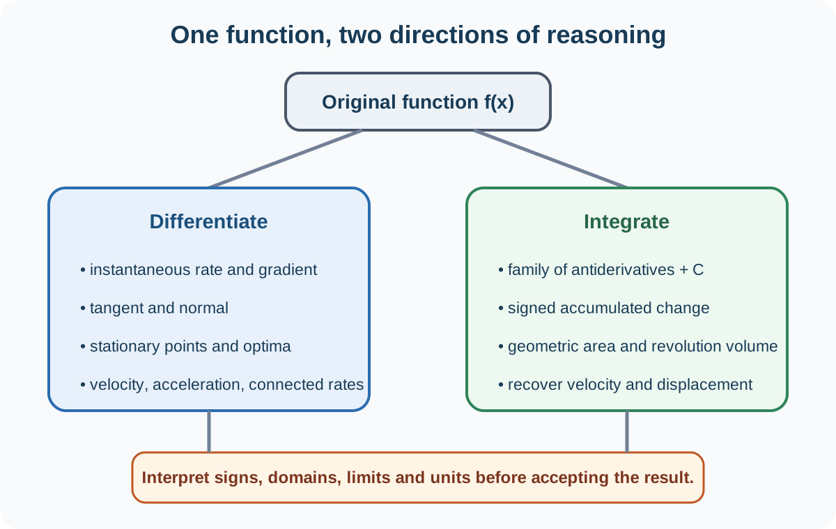
Calculus connects local change with accumulated change. Pearson International GCSE Further Pure Mathematics (4PM1) includes differentiation and integration of sums of powers, sine, cosine and exponential functions; product, quotient and simple chain rules; tangents, normals and stationary points; maxima and minima; kinematics; areas and volumes of revolution; connected rates; and the small-increment approximation. Integration of 1/x is explicitly excluded from this topic, so it is not treated as a required rule here.
1. What a derivative means
For y = f(x), the derivative dy/dx is the limiting gradient of the curve at a point. It measures instantaneous output change per unit input change. Its units are output units divided by input units. A positive derivative means the function is locally increasing, a negative derivative means it is decreasing, and a zero derivative identifies a stationary point candidate.
The second derivative d²y/dx² measures how the first derivative changes. It describes local curvature and can help classify stationary points. A positive second derivative at a stationary point indicates a local minimum; a negative value indicates a local maximum. If it is zero, the test is inconclusive and a sign analysis of the first derivative or another argument is needed.
For a small change dx,
dy ≈ (dy/dx)dx.
This linear approximation uses the tangent line to estimate the corresponding change in y. It is most reliable when dx is small and the derivative does not vary rapidly nearby. The symbol indicates approximation, not exact equality.
2. Core differentiation rules
For a constant a and rational power n,
d/dx(axⁿ) = anxⁿ⁻¹.
Differentiate sums term by term. A constant differentiates to zero. Negative and fractional powers use the same rule wherever the original expression and derivative are defined.
The required standard derivatives include:
d/dx(sin ax) = a cos ax;
d/dx(cos ax) = -a sin ax;
d/dx(eᵃˣ) = aeᵃˣ.
Angles in calculus formulas are interpreted in radians. The internal multiplier a appears because of the chain rule.
For a product y = uv,
dy/dx = u(dv/dx) + v(du/dx).
Both terms are required. For a quotient y = u/v,
dy/dx = [v(du/dx) - u(dv/dx)]/v².
Check this topic from memory
Attempt the matching topic bank before reopening the notes. Use each missed idea to decide what to review next.
Preserve the numerator order and square the entire denominator. Simplifying an algebraic quotient before differentiating may be easier, but only when the simplification is valid on the relevant domain.
For a composite function y = f(g(x)), the chain rule multiplies the outer derivative by the inner derivative. In simple power form,
d/dx[(g(x))ⁿ] = n[g(x)]ⁿ⁻¹g'(x).
Identify inner and outer functions before differentiating. A missing inner derivative is one of the most common calculus errors.
3. Tangents and normals
At x = a, calculate the point (a, f(a)) and tangent gradient f'(a). The tangent equation is
y - f(a) = f'(a)(x - a).
The normal is perpendicular to the tangent. If the tangent gradient is non-zero and finite, its gradient is -1/f'(a). A horizontal tangent has a vertical normal, and a vertical tangent needs separate treatment because its gradient is undefined.
Always use the point on the original curve, not a point inferred from the derivative graph. Substitute the point into the completed line equation as a check. If a tangent must also pass through another given point, use that condition to solve for the contact coordinate.
4. Stationary points and optimization
Stationary points satisfy f'(x) = 0. Solve this equation, then substitute each solution into f to obtain full coordinates. A stationary point may be a local maximum, local minimum or stationary point of inflection.
Classification methods include:
first-derivative signs: positive to negative gives a maximum; negative to positive gives a minimum; no sign change suggests a stationary inflection;
second derivative: f''(a) < 0 gives a maximum and f''(a) > 0 gives a minimum;
structural reasoning, such as a completed square or known domain endpoint.
Optimization in context begins before differentiation. Define the variable, write the target quantity as a function of one variable, and state its feasible domain. Solve stationary conditions, but also inspect endpoints where the context imposes a closed interval. Justify the selected maximum or minimum, give units, and reject algebraic values that violate physical restrictions.
5. Integration
Integration reverses differentiation. For n ≠ -1,
∫ axⁿ dx = [a/(n + 1)]xⁿ⁺¹ + C.
The condition matters because integration of 1/x is outside the specified rule. The constant C represents the family of antiderivatives with the same derivative. An initial condition determines it.
Required trigonometric and exponential results follow by reversal:
∫ sin ax dx = -(1/a)cos ax + C;
∫ cos ax dx = (1/a)sin ax + C;
∫ eᵃˣ dx = (1/a)eᵃˣ + C, for non-zero a.
Differentiate an antiderivative mentally to check signs and factors.
A definite integral uses limits and produces a number:
∫ from a to b of f(x) dx = F(b) - F(a),
where F' = f. It gives signed area: regions below the horizontal axis contribute negatively. Geometric area requires splitting at roots or intersections and making each contribution positive. Area between curves is found from top function minus bottom function on each interval.
6. Volumes of revolution
When the region under y = f(x) from x = a to x = b rotates about the horizontal axis, the disc method gives
V = π∫ from a to b of [f(x)]² dx.
The radius is the vertical distance to the axis, so it must be squared. If the axis of rotation is vertical and the curve is described as x = g(y), integrate π[g(y)]² with respect to y over the corresponding limits. Pearson specifies revolution about coordinate axes.
If a region lies between two curves and rotates to form washers, the cross-sectional area is π(outer radius² - inner radius²). Identify radii geometrically before integrating. Volumes have cubic units, whereas areas have square units.
7. Linear kinematics
For displacement s(t) along a line,
v = ds/dt and a = dv/dt = d²s/dt².
Differentiate displacement to obtain velocity and acceleration. Integrate acceleration to obtain velocity, then integrate velocity to obtain displacement, using initial conditions to determine constants.
Velocity is directed and may be negative. Speed is |v|. A particle is instantaneously at rest when v = 0, but this does not necessarily mean it remains stationary. Direction changes when velocity changes sign. Total distance travelled requires splitting the time interval at every direction change and adding the magnitudes of displacement changes. Net displacement can be smaller because opposite movements cancel.
8. Rates and connected rates
If quantities depend on time, connect them through the chain rule. For a volume V depending on radius r,
dV/dt = (dV/dr)(dr/dt).
Write the geometric relationship first, differentiate with respect to time, then substitute values at the specified instant. Units help check the direction of the relationship. A decreasing quantity has a negative rate, even if the question later asks for the positive magnitude of decrease.
Do not substitute numerical dimensions too early if they are changing. Differentiation must act on variables before an instantaneous value replaces them. If several dimensions vary, every time-dependent term contributes through product or chain rules.
Worked example: optimization and verification
A rectangle has its base on the horizontal axis and its upper corners on the parabola y = 12 - x², symmetrically placed at x = ±x, where 0 < x < √12. Find the rectangle's maximum area. Its width is 2x and height is 12 - x², so A(x) = 2x(12 - x²) = 24x - 2x³. Differentiate: A'(x) = 24 - 6x². Setting this to zero gives x² = 4, hence the admissible value x = 2. The second derivative is A''(x) = -12x, so A''(2) = -24 < 0 and the stationary value is a local maximum. The area is A(2) = 48 - 16 = 32 square units. At the domain endpoints the limiting area is zero, so the interior maximum is also the absolute maximum for the stated configuration.
Common misconceptions and how to correct them
Dropping the inner derivative. Identify the composite layers and multiply by the derivative of the inner function.
Writing only one term in the product rule. Differentiate each factor in turn while retaining the other.
Reversing the quotient-rule numerator. Keep denominator times derivative of numerator minus numerator times derivative of denominator.
Using the tangent gradient for the normal. Take the negative reciprocal, with separate handling for horizontal or vertical cases.
Assuming every stationary point is an extremum. Classify it using derivative signs, second derivative or structural reasoning.
Ignoring endpoints in optimization. A stationary point alone does not prove the absolute optimum on a restricted domain.
Forgetting the integration constant. Include C for indefinite integration and determine it from any condition.
Using the power rule for x⁻¹. The stated integration rule excludes n = -1; do not divide by zero in the new exponent.
Treating a definite integral as always positive area. Split at sign changes and add magnitudes for geometric area.
Confusing velocity with speed or displacement with distance. Use signs for direction and split at velocity zeros for total distance.
Substituting changing dimensions before differentiating connected rates. Differentiate the variable relationship first, then use instantaneous values.
Forgetting to square the radius in a volume of revolution. Cross-sectional disc area is πr², not πr.
Assessment guidance
State the function and relevant domain before differentiating an application. Show derivative rules clearly enough that product, quotient and chain factors can be followed. For stationary points, provide both coordinates and an explicit classification justification. Tangent and normal answers need the contact point and a line equation, not only a gradient. In integration, retain exact antiderivatives, include C when limits are absent, and substitute upper minus lower limits with brackets. Split area or distance calculations wherever signs change. For kinematics, label displacement, velocity, speed and acceleration with units. For connected rates, write the relationship, differentiate with respect to time and substitute only afterward. Check the final dimensions: gradients are rates, areas are squared and volumes are cubed.
Retrieval practice
From memory, write the power, product, quotient and chain rules plus the required sine, cosine and exponential derivatives. Explain three ways to classify a stationary point. Then connect differentiation and integration to tangent lines, signed area, volume of revolution, linear kinematics, connected rates and the approximation dy ≈ (dy/dx)dx, stating one essential check for each.