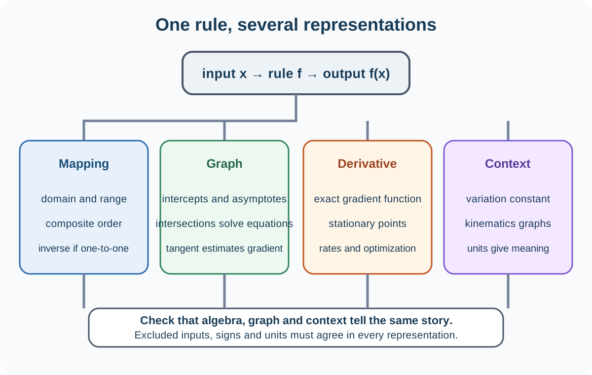
A function assigns exactly one output to each input in its domain. Pearson Edexcel International GCSE Mathematics B (4MB1) develops functions as mappings, notation, domain and range, composites and inverses; specified forms of direct and inverse variation; Cartesian coordinates and straight lines; polynomial and reciprocal graphs; graphical gradients; differentiation of integer powers; stationary points and rates; and applications to linear kinematics. These ideas belong together because a formula, graph and derivative are three views of the same relationship.
1. Functions and mappings
A relation is a function when every permitted input has one output. Different inputs may share an output, but one input cannot map to two different outputs. A mapping diagram makes this condition visible.
The notation f(x) means the output of function f at input x. The mapping notation f: x ↦ 2x + 3 states the rule. It does not mean f multiplied by x. To evaluate f(-2), substitute the complete input using brackets.
An equation such as y² = x does not define y as one real-valued function of x unless a branch is selected, because most positive inputs give two possible values of y. By contrast, y = √x uses the principal non-negative root and is a function on x ≥ 0.
2. Domain and range
The domain is the allowed set of inputs. The range is the set of outputs actually produced. Restrictions may be stated or arise from the rule. A denominator cannot be zero; an even root needs a non-negative radicand for a real-valued function.
For f(x) = 1/x, the real domain excludes zero and the range also excludes zero. For g(x) = √(x - 4), the real domain is x ≥ 4 and the range is g(x) ≥ 0. Pearson does not set questions on continuity here, but it expects excluded domain values to be recognised.
A graph displays domain horizontally and range vertically. Open endpoints or holes indicate excluded values. Never infer the range from an algebraic rule without considering the given domain; a restriction can change the outputs available.
3. Composite functions
The composite fg means “do g first, then f”, so (fg)(x) = f(g(x)) under Pearson's convention. Work from the inside outward. If f(x) = 2x + 1 and g(x) = x², then fg(x) = 2x² + 1, while gf(x) = (2x + 1)². Composition is not generally commutative.
Check this topic from memory
Attempt the matching topic bank before reopening the notes. Use each missed idea to decide what to review next.
The domain of a composite needs two checks: x must belong to the domain of the inner function, and its output must belong to the domain of the outer function. For example, if the outer function contains a reciprocal, inner outputs that equal zero must be excluded.
When evaluating a composite at a number, calculate the inner output first and feed that exact result into the outer function. Keep notation explicit so intermediate outputs are not confused with products.
4. Inverse functions
An inverse function reverses a one-to-one function. If f(a) = b, then f⁻¹(b) = a. The superscript -1 denotes inverse function, not reciprocal: f⁻¹(x) is generally not 1/f(x).
To find an inverse algebraically, write y = f(x), interchange x and y, then solve for y. State any domain restriction needed to make the original function one-to-one. A quadratic on all real inputs has no inverse function because horizontal lines can meet it twice, but restricting it to one side of its turning point can produce one.
The graphs of a function and its inverse reflect in y = x. Their domains and ranges swap. Composition checks the result: f(f⁻¹(x)) = x on the inverse's domain and f⁻¹(f(x)) = x on the original domain.
5. Direct and inverse variation
Variation statements contain an unknown constant k. The official 4MB1 forms include direct and inverse proportionality involving x, x², x³ and √x. Examples are:
y ∝ x, so y = kx;
y ∝ x², so y = kx²;
y ∝ 1/x³, so y = k/x³;
y ∝ √x, so y = k√x;
y ∝ 1/√x, so y = k/√x.
Use one known pair to determine k, then apply the model. The constant carries units needed to make the relationship dimensionally consistent. A direct-proportion graph of y against the stated power of x passes through the origin; an added constant would describe a linear relationship, not direct proportion.
For inverse variation, zero is excluded where it makes the denominator zero. Compare ratios or products to check a result: if y ∝ 1/x², then yx² should remain constant.
6. Coordinates and straight lines
Rectangular Cartesian coordinates locate points as ordered pairs. The gradient between A(x₁, y₁) and B(x₂, y₂) is (y₂ - y₁)/(x₂ - x₁) when the horizontal change is non-zero.
The equation y = mx + c describes a non-vertical straight line with gradient m and vertical intercept (0, c). Parallel non-vertical lines share a gradient. The equation of a line through a known point can be formed with y - y₁ = m(x - x₁), then rearranged if required.
At the intersection of two graphs, both equations have the same x and y. Therefore intersections solve simultaneous equations graphically. Read estimates only to precision supported by the graph scale.
7. Polynomial and reciprocal graphs
Pearson specifies graphical treatment of expressions selected from
y = Ax³ + Bx² + Cx + D + E/x + F/x²,
with numerical constants and at least three constants zero. This produces manageable combinations of cubic, quadratic, linear, constant and reciprocal terms rather than requiring every feature at once.
Construct a value table across a suitable domain, including points near turning points or asymptotes. Plot accurately and join with a smooth curve consistent with the function family. For reciprocal terms, exclude x = 0 and do not draw through a vertical asymptote. Polynomial roots are horizontal-axis crossings or tangencies. A cubic's leading term controls its opposite end behavior.
Use intersections to solve equations. Rearrange an equation so each side can be drawn as one graph, or draw the function and a comparison line. Record all intersections in the requested interval.
8. Graphical gradients
The gradient of a curve at a point is estimated by drawing a tangent that touches locally and follows the curve's direction. Choose two well-separated, readable points on the tangent, not necessarily on the original curve, and calculate rise over run.
A larger triangle reduces the proportional effect of plotting and reading errors. Include axis scales and units. A tangent drawn too short or as a chord through neighboring curve points can give a biased estimate.
The sign of the tangent gradient describes increasing or decreasing behavior. A horizontal tangent has gradient zero and marks a stationary point candidate.
9. Differentiation and stationary points
For an integer power,
d/dx(axⁿ) = anxⁿ⁻¹.
Differentiate sums term by term and constants to zero. This rule handles positive, zero and negative integer powers wherever the original function is defined. It does not include product, quotient or general chain rules in the stated 4MB1 Functions table, so those should not be assumed when choosing an examination method.
The derivative dy/dx gives the exact gradient function. At x = a, substitute a to obtain the curve gradient. Stationary points satisfy dy/dx = 0. Find their coordinates by substituting the resulting x values into the original function.
Classify a stationary point by checking the derivative sign on either side or relating the calculation to the graph. Positive-to-negative change gives a local maximum, negative-to-positive gives a local minimum, and no sign change may indicate a stationary point of inflection.
Optimization requires a model and domain. Form the target function, differentiate, solve the stationary condition and justify whether it is a maximum or minimum. Check endpoints when the variable is restricted.
10. Linear kinematics and practical rates
For displacement s(t) along a line, velocity is v = ds/dt and acceleration is a = dv/dt. Velocity is directed; speed is its non-negative magnitude. A particle changes direction when velocity changes sign, not merely when acceleration is zero.
On a displacement-time graph, gradient is velocity. On a distance-time graph, gradient is speed and should not be negative under the usual accumulated-distance meaning. On a speed-time graph, gradient is acceleration and area represents distance travelled. Interpret axis labels before assigning meaning.
Practical rate questions use the same derivative idea: output change per unit input. State units and interpret signs. Graphical and differentiated answers should agree within plotting accuracy.
Worked example: composite, inverse and domain
Let f(x) = 3x - 4 and g(x) = 1/(x + 2). Find fg(x) and its domain, then find f⁻¹(x) and verify one inverse composition. Since Pearson's fg means apply g first, fg(x) = f(g(x)) = 3/(x + 2) - 4. Its domain excludes x = -2, where g is undefined. For the inverse, write y = 3x - 4, swap variables to obtain x = 3y - 4, and solve: y = (x + 4)/3. Thus f⁻¹(x) = (x + 4)/3. Checking, f(f⁻¹(x)) = 3[(x + 4)/3] - 4 = x. This verification also demonstrates why f⁻¹ is not the reciprocal 1/(3x - 4).
Common misconceptions and how to correct them
Treating a function as any relation. Each domain input must have exactly one output.
Reading fg left to right as “do f first”. Under Pearson's convention, evaluate g first, then f.
Ignoring the outer function's domain in a composite. Inner outputs must be valid outer inputs.
Equating an inverse function with a reciprocal. Find the inverse by swapping input and output and solving.
Finding an inverse without making the function one-to-one. Apply a domain restriction when required.
Leaving out the variation constant. Replace proportionality with an equation containing k.
Calling y = kx + c direct proportion when c ≠ 0. Direct proportion passes through the origin.
Joining a graph across an excluded reciprocal input. Keep branches separated at vertical asymptotes.
Using curve points instead of tangent points for a graphical gradient. Calculate from two points on the drawn tangent.
Differentiating a constant as itself. Its rate of change is zero.
Assuming every stationary point is a maximum or minimum. Check derivative signs or the graph.
Confusing velocity and speed. Velocity has direction and may be negative; speed does not.
Reading graph area without checking axes. Area meaning depends on the plotted quantities and their units.
Assessment guidance
State domains before composing or inverting functions, and retain excluded inputs throughout simplification. Write composite substitutions in nested form to show operation order. For inverses, demonstrate the swap-and-solve method and mention any one-to-one restriction. In variation questions, find k before predicting another value and check the constant relationship. Graphs need sensible scales, accurate points, smooth family-appropriate curves and labelled asymptotes or stationary features. A graphical gradient should show a tangent and a large calculation triangle. In differentiation, display the derivative, stationary equation, coordinates and classification. Kinematics answers need correct graph interpretation, direction language and units. Use an algebraic, graphical or physical check before accepting the result.
Retrieval practice
Define function, domain and range, then calculate two non-commuting composites and an inverse with a domain check. Write all specified direct and inverse variation forms. Sketch representative straight-line, quadratic, cubic and reciprocal graphs, estimate one tangent gradient, differentiate an integer-power sum, classify its stationary points, and interpret displacement-time and speed-time graphs.